Comments on Supernovae
Comments on Supernovae. Riess 2004 sample of SNIa Comments on SNIa systematics Next SNIa surveys Some Kosmoshow analysis of present SNIa data. Charling TAO April 2004, Toulouse. SN Ia 2004 : Riess et al, astro-ph 0402512. 183 SNIa selected Gold set of 157 SN Ia.

Comments on Supernovae
E N D
Presentation Transcript
Comments on Supernovae Riess 2004 sample of SNIa Comments onSNIa systematics NextSNIa surveys SomeKosmoshow analysisof present SNIa data Charling TAO April 2004, Toulouse
SN Ia 2004 : Riess et al, astro-ph 0402512 183 SNIa selected Gold set of 157 SN Ia Fits well the concordance model : c2= 178 /157 SNe Ia
SNIA 2004: Riess et al,astro-ph 0402512 16 new SNIA with HST(GOOD ACS Treasury program) 6 / 7 existing with z >1.25 + Compilation (Tonry et al. 2003): 172 with changes… * Knop et al, 2003, SCP : 11 new 0.4 < z < 0.85 reanalysis of 1999 Perlmutter et al. *15 / original 42 excluded:inaccurate colour measurements and uncertain classification * 6 /42 and 5/11: fail « strict SNIA » sample cut * Barris et al, 2003, HZT: 22 newvarying degrees of completeness on photometry and spectroscopy records * Blakesly et al, 2003 : 2 with ACS on HST • * Low z : 0.01 < z < 0.15 • Calan-Tololo (Hamuy et al., 1996) : 29 • CfA I (Riess et al. 1999): 22 • CfA II (Jha et al, 2004b): 44 (not published yet)
Determination of Cosmological parameters w=p/r w= w0+w’ z Riess et al, astro-ph 0402512
Determination of acceleration Riess et al, astro-ph 0402512
New physics? • Cosmological constant • Dark Energy: Dynamical scalar fields, quintessence…. General equation of state p=w r r = R-3(1+w) Perhaps a bit early !!! « Experimentalist » point of view…
Constraints on cosmological parameters Dm= 0.2 - 0.3 effect!
Systematic error on magnitude 3 fit with no prior Use Kosmoshow: an IDL program by A. Tilquin! marwww.in2p3.fr/~renoir/kosmoshow.html 20% calibration error on intermediate fluxes gives no cosmological constant
Riess gold set sensitivity Kosmoshow, A. Tilquin
A Dm=0.27 shift of low z data Use Kosmoshow: an IDL program by A. Tilquin! Shift z <0.15 data by Dm= 0.27 Wm= 0.43 +/-0.2 and WL= 0 +/-0.34 • No need for L • But Universe is not flat!
The “classical” observation method A 3 steps method: • Discovery: subtraction of an image with a reference one. • Supernova type identification and redshift measurement: spectrum. • Photometric follow-up: light curve. Final analysis: Hubble diagram.
The Hubble diagram Less luminous/z => Accelerated expansion less matter or more dark energy Too luminous/z => Slowed down expansion => deceleration More matter, less dark energy Absolute magnitude m(z) = M + 5 log (DL(z,WM,WL))-5log(H0)+25
Magnitude at maximum mag • Light Curve in local reference frame – K correction • Galactic extinction correction - Standardisation methods : stretch (SCP), MLC2k2 (HiZ), Dm15, ... light curve
Standardisation: stretch method Before: mB After : mBcor = mB – a (s-1)
Precision on the magnitude at the maximum Stretch uncorrected Stretch corrected Precision on the magnitude dominated by intrinsic dispersion: dmint 0.15
Fit cosmological parameters • From Hubble diagram, fit best cosmological model agreeing with observations. • Determine dark energy parameters WL, ou (WX, w, w’) and matter density WM
Spectroscopy needed • SN Ia Identification • Spectrum structure • Redshift z measurement • From position of identified lines from spectra SN and/or underlying galaxy
data analysis physics The « classical » method galaxy magnitude z(redshift) Images Hubble + identification. Spectra Ia
Systematic effects Extragalactic environment local Supernova environment Normal Dust absorption Lensing Grey Dust SN evolution reduction/correlations SNIa contamination Selection bias Inter calibration filters
Systematic effects • SN evolution • Internal extinction not negligible in spiral galaxies • Corrections for peculiar velocity effects • Grey dust • Lensing • Rowan-Robinson astro-ph/021034 • Perlmutter & Schmidt 0303428 • Observational problems • Standardisation method • Light curve fitting • Subtractions • Calibrations • Atmospheric corrections • K-corrections • Selection bias • Heterogeneity of SN data • SNIa identification
Redshift calibration Le flux est intégré sur un filtre pour un point de photométrie • Spectrum is dilated by (1+z) : • The integrated flux in a filter is l Shifted. • Filters responses are not flat • Sometimes, need different filters • Correct for differences systematic effects
SNIa sample contamination Need strict selection criteria Gold sample is probably well selected
Supernovæ identification Ca H&K SiII 4100 With Spectra Main stamp of the SNe Ia: Si II at 6150 Å: Hardly observable beyond z > 0.4-0.5. Otherwise, search for features in the range 3500-5500 Å (supernova rest frame): Ca H&K, SiII at 4100 Å, SII, … Simulation of a SN Ia spectrum at z0,5
Atmospheric transmission (ground) Reduction of transmission in visible Absorption water & O2 reduce visibility in IR . Seeing + weather + moon + field not always visible absorption Reduced efficiency Not homogeneous filters Redshift dependent !!!
Dependence on SN Environment Blue have a lower metallicity Can be seen further
Supernovae evolution Peak magnitude can change • Explosion changes with environment • Difference of chemical elements around SN • Depends on galaxy morphology, age, type,… Sullivan et al (2002) SCP SNIa host galaxy morphological classification Not a large effect, but statistics are low
Extinction and Dust • Extinction by dust from Our or SN galaxy • Correction factor to the magnitude • A = R* E(B-V) • Measurements in many filters • Select minimal dust regions ? Before extinction Rv=3.1 +/- 0.3 for OUR galaxy Very large correction After correction • Grey dust:not well known, intergalactic,?
A strong limit on grey dust? Peerels, Tells, Petric, Helfand (2003) • A 24.7 hr Chandra exposure of QSO 1508-5714 z=4.3 shows no dust scattering halo • Upper limit on mass density of large grained (>1mm) intergalactic dust: Wdust < 2 10-6
Dust and evolution ? Sensitivity to dark energy decrease for z > 0.6 Dust : Homogeneous gray intergalactic dust? Galactic dust responsible for extinction? • Evolution: shift due to progenitor • mass? • metallicity? • Ni distribution? • Other effects? Is there a region of deceleration?Needs to go to z> 1
Systematics Effect of de/amplification
SN demographics studies Understand environment To classify and correct Need precise measurements with statistics Perlmutter
Summary • Ideally • Many SN for a negligible statistical error and study • of systematic conditions. wide field • Detect deceleration zone (z>1) measure in IR • (or have large local UV sample for SNIa identification) • Control the correction precision for SNIA • standardisation (environment and measurement corrections) • Control non corrected systematic effects to the same level • Very precise light curves and spectra to determine • the explosion parameters, at all distances.
Hubble diagrams: Space vs ground Ground limitation at z around 1 due to atmosphere ground simulation space
Advantage of space same observation in space and from ground • More galaxy surface density • Less impact from a more constant PSF • More information on shape Optimisation of mission
SNAP a dedicated satellite Large statistics: 2000 Sne Ia/yr redshift to z<1.7, Minimal selection Ia identification 2m wide field telescope
Mission : % level Science • Measure M and • Measure w and w (z) Systematics Requirements Statistical Requirements • Identified and proposed systematics: • Measurements to eliminate / bound each one to +/–0.02 mag • Sufficient (~2000) numbers of SNe Ia • …distributed in redshift • …out to z < 1.7 Data Set Requirements • Discoveries 3.8 mag before max • Spectroscopy with S/N=10 at 15 Å bins • Near-IR spectroscopy to 1.7 m • • • Satellite / Instrumentation Requirements • ~2-meter mirror Derived requirements: • 1-square degree imager • High Earth orbit • Spectrograph • ~50 Mb/sec bandwidth (0.35 m to 1.7 m) • • •
SNAP goals reach 1 to 2 % on cosmological parameters • Need same precision on extracted magnitude • Fit the magnitude on light curve after corrections of stretch, galactic extinction, K-corrections, everything that modifies luminosity • Study models and parameter extraction • Determine camera properties
data analysis physics SNAP: Observation method The same !! But optimised for systematics galaxy magnitude z(redshift) Images Hubble + same spectra, allows identification. M , L Spectra Ia SiII
SNAP SNIa strategy Discovery maximum 2 days (RF) after explosion ( max + 3.8 magnitude), Ligth curve:At least 10 points in photometry until plateau (+2.5 m) Spectrum very precise at maximum (identification, systematics, calibration)
SNAP survey Hubble Deep Field Observe repeatedly same sky area Wide field !! • Surveys: • Supernova Survey: • 2X7,5 sq. deg. • 2X16 months • R<30.4 (9 bands) • Weak Lensing Survey • 300 sq. deg. • 0.5-1 year • R<28.8 (9 bands) Supernova Survey Weak Lensing Survey Each field is est observed ~4 days All images are cumulated
Light curves Multi band Photometry Peak measurement 2 % K correction Selection bias Very precise measurement of beginning and end of light curve
Simulated SNAP Light Curves z=0.8 z=1.0 z=1.4 z=1.2 z=1.6 Rest B-band Rest V-band Rest R-band Rest B-band Rest V-band