Computational intelligence for data understanding
Computational intelligence for data understanding. Włodzisław Duch Department of Informatics, Nicolaus Copernicus University , Toru ń , Poland Google: W. Duch Best Summer Course ’08. What is this tutorial about ? How to discover knowledge in data;

Computational intelligence for data understanding
E N D
Presentation Transcript
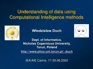
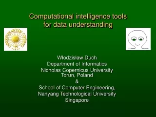
Computational intelligence for data understanding Włodzisław Duch Department of Informatics, Nicolaus Copernicus University, Toruń, Poland Google: W. Duch Best Summer Course’08
What is this tutorial about ? How to discover knowledge in data; how to create comprehensible models of data; how to evaluate new data; how to understand what CI methods do. Plan • AI, CI & Data Mining. • Forms of useful knowledge. • Integration of different methods in GhostMiner. • Exploration & Visualization. • Rule-based data analysis . • Neurofuzzy models. • Neural models, understanding what they do. • Similarity-based models, prototype rules. • Case studies. • DM future: k-separability and meta-learning. • From data to expert systems.
Artificial Intelligence: symbolic models of knowledge. Higher-level cognition: reasoning, problem solving,planning, heuristic search for solutions. Machine learning, inductive, rule-based methods. Technology: expert systems. AI, CI & DM • Computational Intelligence, Soft Computing: • methods inspired by many sources: • biology – evolutionary, immune, neural computing • statistics, patter recognition • probability – Bayesian networks • logic – fuzzy, rough … • Perception, object recognition. • Data Mining, Knowledge Discovery in Databases. • discovery of interesting patterns, rules, knowledge. • building predictive data models.
CI definition Computational Intelligence. An International Journal (1984) + 10 other journals with “Computational Intelligence”, D. Poole, A. Mackworth & R. Goebel, Computational Intelligence - A Logical Approach. (OUP 1998), GOFAI book, logic and reasoning. • CI should: • be problem-oriented, not method oriented; • cover all that CI community is doing now, and is likely to do in future; • include AI – they also think they are CI ... CI: science of solving (effectively) non-algorithmizable problems. Problem-oriented definition, firmly anchored in computer sci/engineering. AI: focused problems requiring higher-level cognition, the rest of CI is more focused on problems related to perception/action/control.
What can we learn? Good part of CI is about learning. What can we learn? Neural networks are universal approximators and evolutionary algorithms solve global optimization problems – so everything can be learned? Not quite ... • Duda, Hart & Stork, Ch. 9, No Free Lunch + Ugly Duckling Theorems: • Uniformly averaged over all target functions the expected error for all learning algorithms [predictions by economists] is the same. • Averaged over all target functions no learning algorithm yields generalization error that is superior to any other. • There is no problem-independent or “best” set of features. • “Experience with a broad range of techniques is the best insurance for solving arbitrary new classification problems.”
What is there to learn? Industry: what happens? Genetics, proteins ... Brains ... what is in EEG? What happens in the brain?
Forms of useful knowledge AI/Machine Learning camp: Neural nets are black boxes. Unacceptable! Symbolic rules forever. • But ... knowledge accessible to humans is in: • symbols, • similarity to prototypes (intuition), • images, visual representations. • What type of explanation is satisfactory? • Interesting question for cognitive scientists but ... • in different fields answers are different!
Forms of knowledge • Humans remember examples of each category and refer to such examples – as similarity-based or nearest-neighbors methods do. • Humans create prototypes out of many examples – same as Gaussian classifiers, RBF networks, neurofuzzy systems. • Logical rules are the highest form of summarization of knowledge, require good linguistic variables. • 3 types of explanation presented here: • exemplar-based: prototypes and similarity; • logic-based: symbols and rules; • visualization-based: maps, diagrams, relations ...
GhostMiner Philosophy GhostMiner, data mining tools from our lab + Fujitsu: http://www.fqs.pl/ghostminer/ • Separate the process of model building (hackers) and knowledge discovery, from model use (lamers) => GhostMiner Developer & GhostMiner Analyzer • There is no free lunch – provide different type of tools for knowledge discovery. Decision tree, neural, neurofuzzy, similarity-based, SVM, committees. • Provide tools for visualization of data. • Support the process of knowledge discovery/model building and evaluating, organizing it into projects. • Many other interesting DM packages of this sort exists: Weka, Yale, Orange, Knime ... 168 packages on the-data-mine.com list!
Wine data example Chemical analysis of wine from grapes grown in the same region in Italy, but derived from three different cultivars. Task: recognize the source of wine sample.13 quantities measured, all features are continuous: • alcohol content • ash content • magnesium content • flavanoids content • proanthocyanins phenols content • OD280/D315 of diluted wines • malic acid content • alkalinity of ash • total phenols content • nonanthocyanins phenols content • color intensity • hue • proline.
Exploration and visualization General info about the data
Exploration: data Inspect the data
Exploration: data statistics Distribution of feature values Proline has very large values, most methods will benefit from data standardization before further processing.
Exploration: data standardized Standardized data: unit standard deviation, about 2/3 of all data should fall within [mean-std,mean+std] Other options: normalize to [-1,+1], or normalize rejecting p% of extreme values.
Exploration: 1D histograms Distribution of feature values in classes Some features are more useful than the others.
Exploration: 1D/3D histograms Distribution of feature values in classes, 3D
Exploration: 2D projections Projections on selected 2D Projections on selected 2D
Visualize data Hard to imagine relations in more than 3D. Use parallel coordinates and other methods. Linear methods: PCA, FDA, PP ... use input combinations. SOM mappings: popular for visualization, but rather inaccurate, there is no measure of distortions. Measure of topographical distortions: map all Xipoints from Rnto xipoints inRm, m < n, and ask: how well are Rij = D(Xi,Xj) distances reproduced by distances rij = d(xi,xj) ?Use m = 2 for visualization, use higher m for dimensionality reduction.
Sequences of the Globin family 226 protein sequences of the Globin family; similarity matrix S(proteini,proteinj) shows high similarity values (dark spots) within subgroups, MDS shows cluster structure of the data (from Klock & Buhmann 1997); vector rep. of proteins is not easy.
Visualize data: MDS Multidimensional scaling: invented in psychometry by Torgerson (1952), re-invented by Sammon (1969) and myself (1994) … Minimize measure of topographical distortions moving the x coordinates. Large distances intermediate local structure as important as large scale
Visualize data: Wine 3 clusters are clearly distinguished, 2D is fine. The green outlier can be identified easily.
Decision trees Simplest things should be done first: use decision tree to find logical rules. Test single attribute, find good point to split the data, separating vectors from different classes. DT advantages: fast, simple, easy to understand, easy to program, many good algorithms. Tree for 3 kinds of iris flowers, petal and sepal leafs measured in cm.
Decision borders Univariate trees: test the value of a single attribute x < a. or for nomial features select a subset of values. Multivariate trees: test on combinations of attributes W.X < a. Result: feature space is divided into large hyperrectangular areas with decision borders perpendicular to axes.
Splitting criteria Most popular: information gain, used in C4.5 and other trees. Which attribute is better? Which should be at the top of the tree? Look at entropy reduction, or information gain index. CART trees use Gini index of node purity (Renyi quadratic entropy):
Non-Bayesian selection Bayesian MAP selection: choose max a posteriori P(C|X) A=0 A=1 P(C,A1) 0.0100 0.4900 P(C0)=0.5 0.0900 0.4100 P(C1)=0.5 P(C,A2) 0.0300 0.4700 0.1300 0.3700 P(C|X)=P(C,X)/P(X) MAP is here equivalent to a majority classifier (MC): given A=x, choose maxCP(C,A=x) MC(A1)=0.58, S+=0.98, S-=0.18, AUC=0.58, MI= 0.058 MC(A2)=0.60, S+=0.94, S-=0.26, AUC=0.60, MI= 0.057 MC(A1)<MC(A2), AUC(A1)<AUC(A2), but MI(A1)>MI(A2) ! Problem: for binary features non-optimal decisions are taken!
SSV decision tree Separability Split Value tree: based on the separability criterion. Define subsets of data Dusing a binary test f(X,s)to split the data into left and right subset D = LS RS. SSV criterion: separate as many pairs of vectors from different classes as possible; minimize the number of separated from the same class.
SSV – complex tree Trees may always learn to achieve 100% accuracy. Very few vectors are left in the leaves – splits are not reliable and will overfit the data!
SSV – simplest tree Pruning finds the nodes that should be removed to increase generalization – accuracy on unseen data. Trees with 7 nodes left: 15 errors/178 vectors.
SSV – logical rules Trees may be converted to logical rules. Simplest tree leads to 4 logical rules: • if proline > 719 and flavanoids > 2.3 then class 1 • if proline < 719 and OD280 > 2.115 then class 2 • if proline > 719 and flavanoids < 2.3 then class 3 • if proline < 719 and OD280 < 2.115 then class 3 How accurate are such rules? Not 15/178 errors, or 91.5% accuracy! Run 10-fold CV and average the results.85±10%? Run 10X and average 85±10%±2%? Run again ...
SSV – optimal trees/rules Optimal: estimate how well rules will generalize. Use stratified crossvalidation for training; use beam search for better results. • if OD280/D315 > 2.505 and proline > 726.5 then class 1 • if OD280/D315 < 2.505 and hue > 0.875 and malic-acid < 2.82 then class 2 • if OD280/D315 > 2.505 and proline < 726.5 then class 2 • if OD280/D315 < 2.505 and hue > 0.875 and malic-acid > 2.82 then class 3 • if OD280/D315 < 2.505 and hue < 0.875 then class 3 Note 6/178 errors, or 91.5% accuracy! Run 10-fold CV: results are 85±10%? Run 10X!
Crisp logic rules: for continuous x use linguistic variables (predicate functions). Logical rules sk(x) şTrue [XkŁxŁX'k], for example: small(x) = True{x|x<1} medium(x) = True{x|xÎ[1,2]} large(x) = True{x|x>2} Linguistic variables are used in crisp (prepositional, Boolean) logic rules: IF small-height(X) AND has-hat(X) AND has-beard(X) THEN (X is a Brownie) ELSE IF ... ELSE ...
Crisp logic is based on rectangular membership functions: Crisp logic decisions True/False values jump from 0 to 1. Step functions are used for partitioning of the feature space. Very simple hyper-rectangular decision borders. Expressive power of crisp logical rules is very limited! Similarity cannot be captured by rules.
Logical rules, if simple enough, are preferable. IF the number of rules is relatively small AND the accuracy is sufficiently high. THEN rules may be an optimal choice. Logical rules - advantages • Rules may expose limitations of black box solutions. • Only relevant features are used in rules. • Rules may sometimes be more accurate than NN and other CI methods. • Overfitting is easy to control, rules usually have small number of parameters. • Rules forever !? A logical rule about logical rules is:
Logical rules are preferred but ... Logical rules - limitations • Only one class is predicted p(Ci|X,M) = 0 or 1; such • black-and-white picture may be inappropriate in many applications. • Discontinuous cost function allow only non-gradient optimization methods, more expensive. • Sets of rules are unstable: small change in the dataset leads to a large change in structure of sets of rules. • Reliable crisp rules may reject some cases as unclassified. • Interpretation of crisp rules may be misleading. • Fuzzy rules remove some limitations, but are not so comprehensible.
Fuzzy inputs vs. fuzzy rules Crisp ruleRa(x) = Q(x-a)applied to uncertain input with uniform input uncertainty U(x;Dx)=1in [x-Dx, x+Dx] and zero outside is true to the degree given by a semi-linear function S(x;Dx): Input uncertainty and the probability that Ra(x) rule is true. For other input uncertainties similar relations hold! For example, triangular U(x): leads to sigmoidal S(x) function. For more input conditions rules are true to the degree described by soft trapezoidal functions, difference of two sigmoidal functions. Crisp rules + input uncertainty fuzzy rules for crisp inputs = MLP !
From rules to probabilities Data has been measured with unknown error. Assume Gaussian distribution: x – fuzzy number with Gaussian membership function. A set of logical rules R is used for fuzzy input vectors: Monte Carlo simulations for arbitrary system => p(Ci|X) Analytical evaluationp(C|X)is based on cumulant function: Error function is identical to logistic f. < 0.02
Rules - choices Simplicity vs. accuracy (but not too accurate!). Confidence vs. rejection rate (but not too much!). p++ is a hit; p-+ false alarm; p+- is a miss.
Rules – error functions The overall accuracy is equal to a combination of sensitivity and selectivity weighted by the a priori probabilities: A(M) = p+S+(M)+p-S-(M) Optimization of rules for the C+ class; accuracy-rejection tradeoff: large g means no errors but high rejection rate. E(M+;g)= gL(M+)-A(M+)= g(p+-+p-+)-(p+++p--)minM E(M;g) minM{(1+g)L(M)+R(M)} Optimization with different costs of errors minM E(M;a) = minM{p+-+ a p-+} = minM{p+(1-S+(M)) -p+r(M)+a [p-(1-S-(M)) -p-r(M)]}
ROC curves ROC curves display S+ vs. (1-S-)for different models (classifiers) or different confidence thresholds: Ideal classifier: below some threshold S+ = 1 (all positive cases recognized) for 1-S-= 0 (no false alarms) . Useless classifier (blue): same number of true positives as false alarms for any threshold. Reasonable classifier (red): no errors until some threshold that allows for recognition of 0.5 positive cases, no errors if 1-S- > 0.6; slowly rising errors in between. Good measure of quality: high AUC, Area Under ROC Curve. AUC = 0.5 is random guessing, AUC = 1 is perfect prediction.
Gaussian fuzzification of crisp rules Very important case: Gaussian input uncertainty. RuleRa(x) = {x>a} is fulfilled byGxwith probability: Error function is approximated by logistic function; assuming error distributions(x)(1- s(x)), fors2=1.7 approximates Gauss<3.5% RuleRab(x) = {b> x>a}is fulfilled byGxwith probability:
Soft trapezoids and NN The difference between two sigmoids makes a soft trapezoidal membership functions. Conclusion: fuzzy logic withsoft trapezoidal membership functions s(x) -s(x-b) to a crisp logic + Gaussian uncertainty of inputs.
Optimization of rules Fuzzy: large receptive fields, rough estimations. Gx – uncertainty of inputs, small receptive fields. Minimization of the number of errors – difficult, non-gradient, but now Monte Carlo or analytical p(C|X;M). • Gradient optimization works for large number of parameters. • Parameterssxare known for some features, use them as optimization parameters for others! • Probabilities instead of 0/1 rule outcomes. • Vectors that were not classified by crisp rules have now non-zero probabilities.
Mushrooms The Mushroom Guide: no simple rule for mushrooms; no rule like: ‘leaflets three, let it be’ for Poisonous Oak and Ivy. 8124 cases, 51.8% are edible, the rest non-edible. 22 symbolic attributes, up to 12 values each, equivalent to 118 logical features, or 2118=3.1035 possible input vectors. Odor: almond, anise, creosote, fishy, foul, musty, none, pungent, spicy Spore print color: black, brown, buff, chocolate, green, orange, purple, white, yellow. Safe rule for edible mushrooms: odor=(almond.or.anise.or.none) Ů spore-print-color = Ř green 48 errors, 99.41% correct This is why animals have such a good sense of smell! What does it tell us about odor receptors?
Mushrooms rules To eat or not to eat, this is the question! Not any more ... A mushroom is poisonous if: R1) odor = Ř (almond Ú anise Ú none); 120 errors, 98.52% R2) spore-print-color = green 48 errors, 99.41% R3) odor = none Ů stalk-surface-below-ring = scaly Ů stalk-color-above-ring = Ř brown 8 errors, 99.90% R4) habitat = leaves Ů cap-color = white no errors! R1 + R2are quite stable, found even with 10% of data; R3and R4may be replaced by other rules, ex: R'3): gill-size=narrow Ů stalk-surface-above-ring=(silky Ú scaly) R'4): gill-size=narrow Ů population=clustered Only 5 of 22 attributes used! Simplest possible rules? 100% in CV tests - structure of this data is completely clear.
Recurrence of breast cancer Institute of Oncology, University Medical Center, Ljubljana. 286 cases, 201 no (70.3%), 85 recurrence cases (29.7%) 9 symbolic features: age (9 bins), tumor-size (12 bins), nodes involved (13 bins), degree-malignant (1,2,3), area, radiation, menopause, node-caps. no-recurrence,40-49,premeno,25-29,0-2,?,2, left, right_low, yes Many systems tried, 65-78% accuracy reported. Single rule: IF (nodes-involved [0,2] Ù degree-malignant = 3 THEN recurrence ELSE no-recurrence 77% accuracy, only trivial knowledge in the data: highly malignant cancer involving many nodes is likely to strike back.
Neurofuzzy system Fuzzy: m(x)=0,1(no/yes) replaced by a degree m(x)[0,1]. Triangular, trapezoidal, Gaussian or other membership f. Feature Space Mapping (FSM) neurofuzzy system. Neural adaptation, estimation of probability density distribution (PDF) using single hidden layer network (RBF-like), with nodes realizing separable functions: M.f-s in many dimensions:
FSM Initialize using clusterization or decision trees. Triangular & Gaussian f. for fuzzy rules. Rectangular functions for crisp rules. Rectangular functions: simple rules are created, many nearly equivalent descriptions of this data exist. If proline > 929.5 then class 1 (48 cases, 45 correct + 2 recovered by other rules). If color < 3.79285 then class 2 (63 cases, 60 correct) Interesting rules, but overall accuracy is only 88±9% Between 9-14 rules with triangular membership functions are created; accuracy in 10xCV tests about 96±4.5% Similar results obtained with Gaussian functions.
Prototype-based rules C-rules (Crisp), are a special case of F-rules (fuzzy rules). F-rules (fuzzy rules) are a special case of P-rules (Prototype). P-rules have the form: IF P = arg minR D(X,R) THAN Class(X)=Class(P) D(X,R) is a dissimilarity (distance) function, determining decision borders around prototype P. P-rules are easy to interpret! IF X=You are most similar to the P=SupermanTHAN You are in the Super-league. IF X=You are most similar to the P=Weakling THAN You are in the Failed-league. “Similar” may involve different features or D(X,P).
P-rules Euclidean distance leads to a Gaussian fuzzy membership functions + product as T-norm. Manhattan function =>m(X;P)=exp{-|X-P|} Various distance functions lead to different MF. Ex. data-dependent distance functions, for symbolic data:
Promoters DNA strings, 57 aminoacids, 53 + and 53 - samples tactagcaatacgcttgcgttcggtggttaagtatgtataatgcgcgggcttgtcgt Euclidean distance, symbolic s =a, c, t, g replaced by x=1, 2, 3, 4 PDF distance, symbolic s=a, c, t, g replaced by p(s|+)