Topic 7: Market Structures
Topic 7: Market Structures. Agenda, Friday 26 th November 2010 A: Supply and Perfect Competition B: Monopoly C: Perfect Competition v. Monopoly D: Oligopoly and Game Theory. A: Supply and Perfect Competition. Firm Supply.

Topic 7: Market Structures
E N D
Presentation Transcript
Topic 7: Market Structures Agenda, Friday 26th November 2010 A: Supply and Perfect Competition B: Monopoly C: Perfect Competition v. Monopoly D: Oligopoly and Game Theory
Firm Supply • How does a firm decide how much to supply at a particular market price? (Firm’s supply curve) • This depends upon the firm’s • goals (e.g. π max, revenue max, zero π, … ); • technology (e.g. w, r, … ); • competitive environment/market structure.
Perfect Competition Assumptions • There are many buyers and sellers, • each seller is (or at least acts as) a price-taker • Homogeneous product • Freedom of entry and exit • Perfect information (consumers know all prices and producers know all input prices/costs)
The Firm’s Short-Run Supply Decision? • Assume each firm is a profit-maximizer • Therefore, each firm chooses its output level by solving: MR = MC But MR = P in perfect competition Therefore P = MC
The Firm’s Short-Run Supply Decision? P At y = ys*, p = MC and MCslopes upwards, y = ys* is profit-maximizing. pe MCs(y) y’ ys* y
The Firm’s Short-Run Supply Decision? P So a profit-maximizing supply level can lie only on the upwards sloping part of the firm’s MC curve. pe MCs(y) y’ ys* y
The Firm’s Short-Run Supply Decision? • The firm will not supply any output if Shut Down Point: P = AVC(y)
The Firm’s Short-Run Supply Decision? Shutdown point P MCs(y) ACs(y) AVCs(y) The firm’s short-runsupply curve y
Short Run Market Supply Curve P Market Supply Curve is the sum of all the firms supply curves (MC) S Q
Perfect Competition: Equilibrium • Short run: (Excess, Abnormal, Supernormal, Economic) Profits or Losses (≤ TVC) possible • Short run → Long run: Profits attracts entry, market supply curve shifts to right, market price falls, zero economic profits in long run equilibrium • Short run → Long run: Losses “attracts” exit, …
Application: Tax Incidence In Perfect Competition Market Supply P PC = PP Market Demand Q No tax: PC = PP (Consumer price = Producer price)
Application: Tax Incidence In Perfect Competition P Market Supply PC This is the tax. PP Market Demand Q The tax creates a wedge between the price firms receive (Pp) and the price consumers pay (Pc). The difference is the tax (which goes to the tax authorities).
Application: Tax Incidence In Perfect Competition P Market Supply PC This is the tax PP Market Demand Q In the short run, the burden of the tax is shared (not necessarily on a 50/50 basis) between consumers and producers.
Application: Tax Incidence In Perfect Competition In the short run, • The producers receives less for the product. • Some firms will continue to produce output at a loss (once the reduced price is covering their average variable costs). • Some firms will experience “excessive” losses and so will exit the market. • The supply curve shifts to the left and the prices consumers and producers face increases.
Application: Tax Incidence In Perfect Competition In the Long Run, • Consumers pay all of the tax (100%) • Producers pay none of tax (0%) • There are no firms making losses left in the market.
Monopoly: Why? • Natural monopoly (economies of scale or density) - utility companies, e.g. electricity or natural gas or cable or rail (transmission) network, household waste collection • Statutory monopoly • a patent; e.g. a new drug • sole ownership of a resource; e.g. a toll bridge • Artificial monopoly, e.g. explicit formation of a cartel, e.g. OPEC
Monopoly: Assumptions • Many buyers • Only one seller i.e. not a price-taker • (Homogeneous product) • Perfect information • Restricted entry (and possibly restricted exit)
Monopoly: Market Behaviour p(y) Higher output y causes alower market price, p(y). D y = Q
Monopoly: Equilibrium P Demand MR y = q = Q
Monopoly: Equilibrium MC P AC y Demand MR
Monopoly: Equilibrium MC Output Decision MC = MR P AC ym y Demand MR
Monopoly: Equilibrium Pm = price MC P AC Pm ym y Demand MR
Monopoly: Equilibrium • Firm = Market • Short run equilibrium diagram = long run equilibrium diagram (apart from shape of cost curves and possibility of exit) • At qm, pm > AC therefore you have excess (economic, supernormal, abnormal) profits • Short run losses are also possible
Monopoly: Equilibrium MC The shaded area is the excess profit P AC Pm ym y Demand MR
Application: Tax Incidence in Monopoly MC curve is assumed to be constant (for ease of analysis) P MC y Demand MR
Application: Tax Incidence in Monopoly • Claim When you have a linear demand curve, a constant marginal cost curve and a tax is introduced, price to consumers increases by “only” 50% of the tax, i.e. “only” 50% of the tax is passed on to consumers. (Similarly, if tax is eliminated, only 50% of price reduction is passed on to consumers.)
Application: Tax Incidence in Monopoly Output decision is as before, i.e. MC = MR So Ybt is the output before the tax is imposed P MCbt ybt y Demand MR
Application: Tax Incidence in Monopoly Price is also the same as before Pbt = price before tax is introduced. P Pbt MCbt ybt y Demand MR
Application: Tax Incidence in Monopoly The tax causes the MC curve to shift upwards P Pbt MCat MCbt ybt y Demand MR
Application: Tax Incidence in Monopoly Price post tax is at Ppt and is higher than before. P Ppt Pbt MCat MCbt ybt yat y Demand MR
Agenda • Societal Welfare/Economic Welfare: Criteria? Consumer Surplus Producer Surplus • Compare Monopoly and Perfect Competition
Economic Welfare • Consumer surplus measures (net) economic welfare from the buyer/consumers’perspective. • Producer surplus measures (net) economic welfare from the seller/producers’perspective.
Consumer Surplus • Consumer surplus is the amount a buyer is willing to pay for a product minus the amount the buyer actually pays. • Consumer surplus is the area below the demand curve and above the market price. A lower market price will increase consumer surplus (provided that the product is still supplied, of course). A higher market price will reduce consumer surplus.
Producer Surplus • Producer surplus is the amount a seller is paid for a product minus the total variable cost of production. A higher market price will increase producer surplus (provided that the product is still demanded, of course). A lower market price will decrease producer surplus. • Producer surplus is equivalent to economic profit in the long run.
Economic Welfare • Economic welfare is (generally) quantified as the sum of consumer surplus and producer surplus, i.e. equal weights are generally assumed. • Alternative relative weights are also possible.
Price A D Supply Consumer surplus Equilibrium price E Producer surplus Demand B C 0 Quantity Equilibrium quantity Consumer Surplus and Producer Surplus: Market Equilibrium
Monopoly v. Perfect Competition MC Price is Ppc P Ppc Qpc Q Demand
Monopoly v. Perfect Competition MC Recall that for monopoly, MR Demand P Output is set where MC=MR Ppc Qm Qpc Q Demand MR
Monopoly v. Perfect Competition MC The monopoly output is less than the perfectly competitive output. P Pm (The monopoly price is higher than the perfectly competitive price.) Ppc Qm Qpc Q Demand MR
Monopoly v. Perfect Competition MC The green area represents the deadweight loss (triangle) of Monopoly P Pm Ppc Qm Qpc Q Demand MR
Oligopoly: Assumptions • Many buyers • Very small number of major sellers ( actions and reactions are very important) • Homogeneous product (usually, but not necessarily) • Complete information (usually, but not necessarily) • Restricted entry (usually, but not necessarily)
Oligopoly & Game Theory: Models • Cournot Competition (1838) (Bertrand Competition (1883)) • Nash Equilibrium (1950s): Game Theory • Oligopoly v. Perfect Competition v. Monopoly • Some examples of Games
1. Cournot Competition • Firms compete in quantities (q1, q2) • Real world examples? • q1 = F(q2) and q2 = G(q1) or more precisely q1 = F(q2e) and q2 = G(q1e) • Aim: Find q1and q2and hence P, i.e. find the equilibrium. • Example: P = a – bQ and Ci = cqi
1. Cournot Competition: Example q2 COURNOT EQUILIBRIUM q1
2. Cournot Competition & Bertrand Competition: Nash Equilibrium Cournot Nash (q1, q2): Firms compete in quantities, i.e. Firm 1 chooses the best q1 given q2 and Firm 2 chooses the best q2 given q1 [Bertrand Nash (p1, p2): Firms compete in prices, i.e. Firm 1 chooses the best p1 given p2 and Firm 2 chooses the best p2 given p1] Nash Equilibrium (s1*, s2*): Player 1 chooses the best s1 given s2* and Player 2 chooses the best s2 given s1*