the sales comparison approach
Sales Comparison Approach (SCA). An appraisal procedure in which the market value established is based on prices paid in actual market transactions and current listingsThe process of analyzing sales of similar recently sold properties in order to derive an indication of the most probable sales price of the subject property being appraised.

the sales comparison approach
E N D
Presentation Transcript
1. The Sales Comparison Approach Dr. Curtis F. Lard
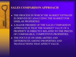
2. Sales Comparison Approach (SCA) An appraisal procedure in which the market value established is based on prices paid in actual market transactions and current listings
The process of analyzing sales of similar recently sold properties in order to derive an indication of the most probable sales price of the subject property being appraised
3. Economic Principles used by the Sales Comparison Approach Competition
Substitution
Supply
Demand
Highest and Best Use
4. Steps in SCA to Valuation Define the Problem�Establish PMV of Subject Property
Select Comparable Market Sales
Make Adjustments to S.P.
Reconcile Value Estimates
Estimate Final Value for S.P.
5. Type of Adjustments Lumps Sum (Location, Neighborhood, etc.)
Linear Trends (Time)
Variable Rates (Size)
Percent Factor & Grades (quality and condition)
6. Items Adjusted Location
Time
Size
Quality Improvements
Water
Minerals
Terms
7. Market Characteristics & Why Adjustments are Needed Heterogeneous product
Few sales occur
Sales are localized
�Lumpy� product
Large Amounts of cash
Inexperienced buyers and sellers
Lack of market information
Location is VERY important
8. Market Assumptions Sellers will not take less than PMV of Similar Property
Buyers will not pay more than PMV of Similar Property.
9. Rules of Thumb Always adjust to the SUBJECT PROPERTY!!!
Any �comp� used should have a minimum effect of .1 on the estimate of PMV for the Subject Property
No �comp� should have more than .5 weight on PMV of Subject Property
These factors help determine weights:
# of Adjustments
Absolute adjustments
10. Ideal �Comps� Adjoins subject property
Same Size
Identical in improvements
Same access and/or problems
Sold yesterday
11. The Sales Comparison Approach Works Where: You can identify market areas
You let the market show differences
12. The Sales Comparison Approach Is Commonly Used For: Residences
Lots
Small businesses
Rural lands
13. Lump Sum Example (Location, Neighborhood, etc.)
14. Lump Sum Example Continued:Sales in Neighborhoods in B/CS
15. Linear Trends Example(11% per year) Estate Settlement as of 6-1-2004
16. Linear Trends Example: Adjustments Adjustment for Comp #2: 2 yrs., 3 mos.
1150 ? 1.11 = 1276.50
1276.50 ? 1.11 = 1416.91
1416.91 ? [(3/12)(11%) + 1] = 1455
Adjustment for Comp #3: 3 mos.
1150 ? [(3/12)(11%) + 1] = 1181
Adjustment for Comp #4: 1 yr., 4 mos.
1250 ? 1.11 = 1387.50
1387.50 ? 1.0367 = 1438
Adjustment for Comp #5: 4 mos.
1295 ? 1.0367 = 1342
17. Linear Trends Example: Conclusions PMV of SP =
.4 (Comp #1)
+ .1(Adjusted Comp #2)
+ .2 (Adjusted Comp #3)
+ .1(Adjusted Comp #4)
+ .2(Adjusted Comp #5)
.4 (1225)
+ .1(1455)
+ .2 (1181)
+ .1(1438)
+ .2(1342)
Present Market Value of Subject Property = 1285/acre
18. Variable Rates Land Size�Price Increases as Size Decreases
19. Percentage Factor�Grade or Quality If interrelated, there could be a compound effect.
20. Sources of Information Acquainted Persons/Community Members
CEA, VoAg Teacher, SCS, ASCS, planners, zone officials, building inspectors
Handlers of farm supplies
Building contractors, farm equipment dealers, farm co-ops, elevator managers, milk plant, LS Mkg.
Persons who sell land or make loans
RE brokers or salesmen, FLB officers, INS, PCA, brokers
Farm Managers, Appraisers, Ag. Consultant
Other sources
Water district, irrigation district, COFC, TREC, USDA publications, US Department of Labor, central appraisal districts
21. Problems with the Sales Comparison Approach Not enough data (common problem)
Cost of gathering data
Quality of data reported
Some trends hold over very limited range
Ranges are subjective
Some relationships are not recognized (industry or courts)
New relationships must stand up in court & the cost of proving is expensive
22. Cash Equivalency Analysis Some sellers give buyers more favorable financing terms than the market conditions. When this happens, the appraiser must make the necessary adjustments in the sales price to compensate for this. The trade-off for favorable financing to the buyer is a higher sales price. Therefore, the following procedure can be used to adjust for this enhancement in the sales price.
23. Cash Equivalency Cash Equivalency: An adjustment for differences in financing a property when sold.
C.E.V = DPM + PWF (Pt)
CEV: Cash Equivalent Value
DPM: Down Payment
PWF: Present Worth Factor
Pt: Annual Payment
AFF = Sales Price � CEV
24. Cash Equivalency Example Typical Market Conditions
20% DPM, 30 yrs, @12% interest
Sale:
100 Acre tract sold for $100,000; 20% DPM; 30-yr. mortgage @ 9% interest.
25. Cash Equivalency Example CEV = DPM + PWF (Pt)
CEV = + ?
CEV = $20,000 + $62,724 = $82,724
AFF = $100,000 � $82,724 = $17,276
Example #2: See notes