XCTL (Explicit Clock Temporal Logic)
XCTL (Explicit Clock Temporal Logic) Real-Time Extension for LTL Qualitative properties responsiveness: “Every stimulus p must be eventually followed by a system response q” invariance: “The system constantly emits signal q” Quantitative properties

XCTL (Explicit Clock Temporal Logic)
E N D
Presentation Transcript
XCTL(Explicit Clock Temporal Logic) Real-Time Extension for LTL
Qualitative properties • responsiveness: “Every stimulus p must be eventually followed by a system response q” • invariance: “The system constantly emits signal q”
Quantitative properties • bounded responsiveness: “Every stimulus p must be followed by a system response q within t time units” • bounded invariant: “The system emits signal q for 2 seconds”
Approaches to Time Quantification First order monadic logic t. p(t) s. q(s) st s t+3 Current time variable: x. □((pT=x ◊(q T x+3)) Bounded operators: □(p ◊[0,3]q) Freeze quantification: □x.(p ◊y.(q y x+3))
XCTL: Syntax Vocabulary: • Propositions: p, q,… • Timing elements: • Time Constants: C = {a, b, c,…} • Timing variables: V = {x, y,…} • Clock variable: T Atomic formulae • Propositions • a + x T, a + x c where: aNat.,{, , } Formulae: • Atomic formulae • p, pq, Op, pUq
Examples • Atomic time expressions: xT, Ty5, x>3 • ((p(xT)) (q(Tx5)))
XCTL Model & Semantics Model for a formula [P,V]*: (0,t0), (1,t1), (2,t2)… where i2P, tiInt s.t. • For all i, titi+1 • nInt j s.t. tjn. Semantics: j |= a+x T iff a+x tj for every : {x} Int. j |= a+x c iff a+x c for every : {x} Int. A model satisfies a formula [P,V] iff 0 |= for every : V Int. * P- set of propositions, V- set of time variables in
Example A model for: ((p(xT)) (q(Tx5)))
Railroad Crossing in XCTL: Assertions • 40 seconds minimal delay between trains. Tin O1,39Tin Tin (x=T) O(Tin (x40T)) • It takes a train 6 seconds to arrive at the signal. Tin O6(AtSignal) Tin(x=T) (AtSignal(x+6=T))
Railroad Crossing in XCTL: Assertions • Trains exit XR within 15 to 25 seconds after passing the signal. (AtSignalTwait) (TwaitPass)O15,25Tout ((AtSignalTwait) (TwaitPass)x=T) (Tout (x+15T)(x+25T))
Railroad Crossing in XCTL: Requirements • Every train that arrives at the signal is allowed to continue beyond the signal within 10 seconds. AtSignal O0,10(Twait) AtSignal (x=T) (Twait (x+10T)) • The gate is open whenever the crossing is empty for more than 10 seconds. O0,10(Tcr0) O10(Open) (x=T) Tcr0U(x+10=T) (Open (x+10=T))
XCTL Closure CL() - is the minimal set that satisfies: • CL(), tt, O(tt)CL() • CL() CL() • UCL() , , O(U)CL() • OCL() CL() • Timing formulae (next slide)
Closure Timing Formulae • Let {a+x}, {c,T}, {, , } • CL() , , CL() • T CL() O( T), ( T)CL() Also, the “difference table”: |CL()| <3||2
Example: Cl((p (T5))) 9. (p(T=5), 10. O(p(T=5), 11. T5, 12. T5, 13. O(T5), 14. (T5) 15. (T5), (T5) 16. tt, ff, Ott 1. (p (T5)), 2. (p (T5)), 3. O(p (T5)), 4. p, 5. T=5, 6. p, 7. (T=5), 8. (p(T=5)),
Atoms A set ACL() such that: • tt, O(tt) A (guarantees infinite models) • for every CL(), A A • for every CL(), A A or A • for every UCL(), UA A or ,O(U)A • for every CL() precisely one of , , A • TA O(T)A • TA (T)A • The difference table w.r.t. A • The set of constraints in A, C(A), is consistent (a solution to a linear system).
Timed Next Relation OA B (A,B)X c A c B =TA =TB or TB
Example: Cl((p (T5))) Atoms Atom#1 (p (T5)), O(p (T5)), T5, (T5) Atom#2 (p (T5)), (p (T5)), p, T=5, (T5) Atom#3 T5, O(T5),
Atom#1 Atom#2 Atom#3 Graph Construction G()(At,X) where At is the set of all atoms that contain , or are accessed from an atom that contains via the X relation
SCS Classification Let C be a strongly connected sub-graph of G() • C is terminal if it has no outgoing edges. • C is self-fulfilling if every atom has a successor within C, and for every pUqA (in C) there is an atom B (in C) such that qB. • C is useless if it is terminal and not self-fulfilling.
Timing Relations between Atoms (A,B)X, C(A)={T1,…,Tk, L1,…,Lm} by definition C(B)={T'1,…,T'k, L1,…,Lm} such that: • if Tj is T then T'j is T • if Tj is T then T'j is T or T • if Tj is T then T'j is T Li are of theform a+x ~ c, and Ti are of the form a+x ~ T.
Lemmas BW-Lemma: If u1,…,un,t' Int satisfy C(B) then there exists tt' such that u1,…,un,t satisfy C(A). FW-Lemma: If A, B belong to a self-fulfilling s.c.s. then C(A)=C(B) and all time constraints in C(A) are of the form T.
BW-Lemma: If u1,…,un,t' Int satisfy C(B) then thereexists tt' such that u1,…,un,t satisfy C(A). Proof • u=u1,…,un |= L1,…,LmC(A), C(B) (t’) • iTC(A)iT | i<TC(B), def. t=i(u) t=i(u)t’. for <TC(A)i- >0C(A)t>(u), sim. for >TC(A). • iTC(A), def El= { i | i<T}, let l=max(l(u)) (l if El= ) Eg={ i | i >T}, let g=min(g(u)) (g if Eg=) g-l>1C(A) g>l+1, let t=l+1 l<t<g. l<TC(A)l<TC(B)l(u)=l<t’ t t'
FW-Lemma: If A, B belong to a self-fulfilling s.c.s. then C(A)=C(B) and all time constraints in C(A) are of the form T. Proof AB, BA {Li} same in A,B & <TC(A)iff <TC(B). Assume =T |>T C(A)(<T)A DC, <TD, but DA <TC(A) !!! • From FW-Lemma: If u1,…,un,t satisfy C(A) then it is a solution forevery atom in a self-fulfilling s.c.s. that contains A.Also, u1,…,un,t' is a solution for every t't.
Fulfilling Paths An infinite path A0,A1,… in G() is called a fulfilling path for if: • For every i, (Ai,Ai+1)X, • For every i, and every pUqAi, there exists some ji such that qAj. • A0
Fulfilling Paths and Satisfiability Theorem: is satisfiable iff there exists a fulfilling path for in G(). Sketch of proof: • if is satisfiable construct the sequence: A0,A1,.. where Ai={ CL() | i |= } Show that is fulfilling path. - Given A0,A1,.. is fulfilling path of . define 0,1,.. s.t.: i={ pAi }. Since is infinite there exists k s.t. all the atoms from k head are contained in a self-fulfilling SCS. Let u1,...un,tk be a solution of Ak, then trace backwards and assign values titk (possible by BW-Lemma). Also by FW-Lemma assign k+1,k+2,.. by tk+1, tk+2,...
Satisfiability Checking Algorithm • Let G0=G(). • repeat with the last defined graph Gi Let C be a useless maximal SCS in Githen define Gi+1=(Wi+1,Xi+1) by: Wi+1=Wi-C Xi+1=Xi(Wi+1Wi+1) until Gi is empty or does not contain anyuseless maximal SCS. • If there is an atom AGi such that A • then report success • else report fail. Theorem: is satisfiable iff the algorithm reports success.
Remarks • The algorithm does not check for complete models(time increases with at most 1 t.u.).. Hence, the Formula (x=T) O(x+2=T) is satisfiable though it does not have a complete model. • The definition of a model does not require time to be non- negative. Hence, the formula (x=T) O(x=-1) is satisfiable but only by a model where t00. In order to restrict models to non-negative clocks we need to augment formulae with a proper constraint p (0T)