Download
1 / 22
220 likes | 256 Vues
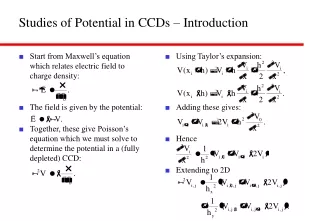
Start from Maxwell’s equation which relates electric field to charge density: The field is given by the potential: Together, these give Poisson’s equation which we must solve to determine the potential in a (fully depleted) CCD:. Using Taylor’s expansion: Adding these gives: Hence

E N D
Start from Maxwell’s equation which relates electric field to charge density: The field is given by the potential: Together, these give Poisson’s equation which we must solve to determine the potential in a (fully depleted) CCD: Using Taylor’s expansion: Adding these gives: Hence Extending to 2D Studies of Potential in CCDs – Introduction
Substitute in Poisson’s equation: Rewrite: Use this to solve iteratively for V. “Tortoise convergence” i.e. sure, but slow! Choosing reasonable initial guess at potential speeds up solution. Need only calculate potential in one pixel if use periodic boundary conditions, e.g. Introduction
Can use different step sizes to reduce time needed for calculation. Start from Taylor expansion again: Adding these expressions and rearranging: Subtracting: Hence Substituting to get the second derivative: Introduction
Now substituting in Poisson’s equation: Rewriting as before: Extending to 2D (variable step size in y coordinate): Introduction
Extension of above should allow determinations of effective gate capacitance. Must determine charge that drive needs to supply in order to change gate voltage. Use Gauss’ law... ...for two different gate voltages, then calculate capacitance: Alternatively, rewrite... ...to give: Hence Q = rDV and C. Introduction
Change grid used to perform calculations. “Large”: 80 x 90 x 40 = 2.9 x 10⁵. “Small”: 32 x 80 x 32 = 1.2 x 10⁵. Potential along buried channel nominal (red) and small (blue) grids. Depth of buried channel: Nominal grid, 0.588 mm. Small grid, 0.582 mm. Potentials opposite shown at grid point closest to above depth. Typical error due to this illustrated by difference between solid and dashed lines. “Small” grid adequate. V mm Check grid size needed
Calculation with 5.2 x 10⁵ grid points (red) and with 1.4 x 10⁵ grid points (blue), i.e. using coarse grid for lower “uninteresting” part of pixel. Large gains in speed possible without compromising accuracy of results. All subsequent calculations performed with coarse grid for lower 90% of pixel. V m Test variable step sizes
Dopant concentrations. Red, at surface 3.6 x 10²² m-3. Yellow, at surface 1.2 x 10²² m-3. Distributions half Gaussian with s = 0.41 mm. Blue, 1 x 10¹⁹ m-3, uniform. “Trees”, 5 mm decreasing to 3 mm. Cross section through gates. Upper section “expanded” due to varying vertical step size. Narrow Christmas Tree
Potential as function of depth under Christmas Tree (red line), under buried channel to side of Christmas Tree (blue dots) and under channel stop (green dashes). Potential along Christmas tree: DV ~ 1.56 V (red, calc. restricted in depth) DV ~ 1.61 V (blue, calc. full depth) V V m m Narrow Christmas Tree
Horizontal section at depth of buried channel. Width of supplementary channel 5 mm decreasing to 3 mm. Potential along Christmas tree: DV ~ 1.54 V V m Double Christmas Tree
Dopant concentrations. Red, 3.6 x 10²² m-3. Yellow, 1.2 x 10²² m-3. Blue, 1 x 10¹⁹ m-3. Cross section through gates. Double Christmas Tree
Horizontal section at depth of buried channel. Width of supplementary channel 4 mm decreasing to 2 mm Potential along Christmas tree: DV ~ 1.66 V V m Narrow Double Christmas Tree
Dopant concentrations. Red, 3.6 x 10²² m-3, s = 0.2 mm. Yellow, 1.2 x 10²² m-3, s = 0.41 mm. Blue, 1 x 10¹⁹ m-3. Cross section through gates. Shallow double Christmas Tree
Horizontal section at depth of buried channel. Potential along Christmas tree: DV ~ 1.56 V V m Shallow double Christmas Tree
Dopant concentrations. Red, 3.6 x 10²² m-3, s = 0.41 mm. Yellow, 1.2 x 10²² m-3, s = 0.2 mm. Blue, 1 x 10¹⁹ m-3. Potential along Christmas tree: DV ~ 1.57 V V m Deep double Christmas Tree
Dopant concentrations. Red, 7.2 x 10²² m-3, s = 0.2 mm. Yellow, 2.4 x 10²² m-3, s = 0.2 mm. Blue, 1 x 10¹⁹ m-3. Cross section through gates. Shallow double Christmas Tree, shallow buried channel
Horizontal section at depth of buried channel (0.34 mm). Potential along Christmas tree: DV ~ 1.67 V V m Shallow double Christmas Tree, shallow buried channel
Dopant concentrations. Red, 15 x 1022 m-3, s = 0.1 mm. Yellow, 5 x 10²² m-3, s = 0.1 mm. Blue, 1 x 10¹⁹ m-3. Cross section through gates. Very shallow narrow double Christmas Tree
Horizontal section at depth of buried channel (0.16 mm). Potential along Christmas tree: DV ~ 1.79 V V m Very shallow double Christmas Tree and buried channel
Dopant concentrations. Red, 15 x 1022 m-3, s = 0.1 mm. Yellow, 5 x 10²² m-3, s = 0.1 mm. Blue, 1 x 10¹⁹ m-3. Cross section through gates. Very shallow double Christmas Tree and buried channel
Horizontal section at depth of buried channel (0.16 mm). Potential along Christmas tree: DV ~ 1.84 V V m Very shallow narrow double Christmas Tree, very shallow buried channel
Calculations Variable step size in grid implemented. Influence of grid size checked: results appear correct for coarse grid, bit of course can’t see detail below “resolution”! Restricting calculation to upper few microns of pixel does not significantly affect shape of potential along buried channel for fully depleted CCDs, but get overall shift if potential of “ground” plane in restricted calc. incorrect. Results For Christmas Tree structure can change depth of buried channel by varying depth and concentration of dopants. Buried channel at depth of ~ 0.6 mm get DV ~ 1.5 V for 2 Vpp clock swing. Buried channel at depth of ~ 0.35 mm get DV ~ 1.8 V for 2 Vpp clock swing. Buried channel at depth of ~ 0.16 mm get DV ~ 1.85 V for 2 Vpp clock swing. Larger asymmetry in potential obtained for narrower Christmas Tree. Summary