Relational Algebra
After this lecture, you should be able to: Understand the differences between SQL (Structured Query Language) and Relational Algebra expressions . Build queries in Relational Algebra. Understand how DBMS’s process the SQL queries. Make simple query optimization .

Relational Algebra
E N D
Presentation Transcript
After this lecture, you should be able to: Understand the differences between SQL (Structured Query Language) and Relational Algebra expressions. Build queries in Relational Algebra. Understand how DBMS’s process the SQL queries. Make simple query optimization. Be ready for Quiz 4 and Complete Assignment 7 (Part I). Relational Algebra
Relational Algebra • Relational algebra deals with a set of relationsclosed under operators. Operators operate on one or more relations to yield a relation. • Algebraic Expressions (a + b) * c (A B) C • Relational algebra is a basis for database query languages.
Characteristics of Relational Algebra • Operational • The order of operations can be specified. • Set-at-a-time • Multiple rows are processed by one operation. • Not too detailed • How to access data is not specified. • Good for query optimization. • Who supplied P2? • SQL Select SName from S, SP where S.S# = SP.S# and P# = 'P2' ; • Relational Algebra SName (S ⋈ (p#=‘P2‘ SP ))
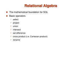
Relational algebra … • Union: A B • Intersection: A B • Difference: A ̶ B • Cartesian Product: S × SP • Division: A / B • Selection: city=‘Rome‘ S • Projection: SName,StatusS • Join: S ⋈ SP • Renamingρ(citypcity) P
Terms: Relational algebra ~ Database Relation ~ Table Attribute ~ Column Tuple ~ Row (Record) Relation schema ~ Structure of table Relation Instance ~ Data of table
Union and Intersection P Q P Q P Q
Union and Intersection: Exercise P Q P Q = ? P Q = ?
Difference (-) Q P P ̶ Q
Difference: Exercise Q P P ̶ Q = ?
Cartesian Product (×) Q P P × Q = {(p, q)|p P and q Q}
Cartesian Product: Exercise Q P P × Q = ?
Selection () R B = 2 R
Get all the information of the suppliers located in Paris. Table S sno | sname | status | city ----------------------------- s1 | Smith | 20 | London s2 | Jones | 10 | Paris s3 | Blake | 30 | Paris s4 | Clark | 20 | London s5 | Adams | 30 | Athens select * from s where city = ‘Paris’; city = ‘Paris‘ S
Projection () R C, AR
What are the S#’s and statuses of the suppliers? Table S sno | sname | status | city ----------------------------- s1 | Smith | 20 | London s2 | Jones | 10 | Paris s3 | Blake | 30 | Paris sno | status ------------ s1 | 20 s2 | 10 s3 | 30 select sno, status from s; sno, statusS
What are the S#’s and statuses of the suppliers located in Paris? Table S sno | sname | status | city ----------------------------- s1 | Smith | 20 | London s2 | Jones | 10 | Paris s3 | Blake | 30 | Paris s4 | Clark | 20 | London s5 | Adams | 30 | Athens sno | status ------------ s2 | 10 s3 | 30 select sno, status from s where city = 'Paris; sno, status(city = ‘Paris‘ S)
Selection and Projection: Exercise Get the names and weights of the green parts. pno pname color weight city ---- ------ ------- ------ ------ p1 nut red 12 London p2 bolt green 15 Paris p3 screw green 17 Rome pname weight ----- ------ bolt 15 screw 17 select pname, weight from p where color = ‘green’; pname, weight(color = ‘green‘ P)
Join P Q B1 ≥ B2(P × Q)
Equijoin Q P B1 = B2(P × Q)
Natural Join (⋈ ) P Q P ⋈ Q
Natural Join: Example S SP S ⋈ SP = ?
Selection, Join, and Projection: Example What are the part numbers of the parts supplied by the suppliers located in Taipei? SQL: select SP.pno from S, SP where S.city = ‘Taipei’ and S.sno = SP.sno; Algebra: pno((S.City=‘Taipei’S)⋈ SP)
Selection, Join, and Projection: Exercise What are the names of the suppliers who supplied green parts? SQL: select sname from P, SP, S where P.color = ‘green’ and P.pno = SP.pno and SP.sno = S.sno; Algebra: sname((pno(color=‘green‘P))⋈ SP ⋈ S)
Subtraction Examples Get the supplier numbers of the suppliers who did not supply red parts. • The supplier numbers of all the suppliers: AS = s# (S) • The supplier numbers of the suppliers who supplied some red parts: RPS = s# (SP ⋈ (Color = ‘Red‘ (P)) • The answer is: AS - RPS
Subtraction Examples (cont’d) Get the names of the suppliers who supplied only red parts. • The supplier numbers of the suppliers who supplied some parts: SS = s# (SP) • The supplier numbers of the suppliers who supplied at least one non-red parts: NRS = s# (SP ⋈ (color <> ‘Red‘ (P)) • The answer is: SName ((SS – NRS) ⋈ S)
Rename (ρ) Ρ(B->B2, 3C2)
Join with Renaming: Example I Get the pairs of the supplier numbers of the suppliers who supply at least one identical part. SQL: select SPX.sno, SPY.sno from SP SPX, SP SPY where SPX.pno = SPY.pno and SPX.sno < SPY.sno Algebra: snox,snoy(snox < snoy ((ρ(snosnox)sno,pnoSP)⋈ (ρ(snosnoy)sno,pnoSP) ) )
Join with Renaming: Example II What are the colors of the parts supplied by the suppliers located in Taipei? Table S Table P sno | sname | sts | city pno | pname | color | wgt | city -------------------------- ---------------------------------- s1 | Smith | 20 | London p1 | nut | red | 12 | London s2 | Jones | 10 | Taipei p2 | bolt | green | 17 | Taipei p3 | screw | blue | 17 | Rome Table SP sno | pno | qty --------------- s1 | p1 | 300 s2 | p3 | 200
Join with Renaming: Example II What are the colors of the parts supplied by the suppliers located in Taipei? SQL: select color From S, SP, P where S.city = ‘Taipei’ and S.sno = SP.sno and SP.pno = P.pno; Algebra: color(S.City=‘Taipei‘(S ⋈ SP ⋈ P)) Joined also by S.city = P.city !
Join with Renaming: Example II (cont’d) Not Correct: color(S.City=‘Taipei‘(S ⋈ SP ⋈ P)) Renamed: color(City=‘Taipei‘ (S ⋈ SP ⋈ρ(citypcity)P)) Optimized: color((pno((sno(City=‘Taipei‘S)) ⋈ SP))⋈ P)
Join Example: Query Plan color ⋈ pno ⋈ sno city=‘Taipei‘S P S SP
SQL Query Processing • An SQL query is transformed into an algebraic form for query optimization. • Query optimization is the major task of an SQL query proccessor. • select A1, A2, … , Am from T1, T2, … , Tn where C is converted to A1, A2, …, AmC (T1 x T2 x … x Tn) and then optimized.
Query Optimization Guidelines • JOIN operations are associative and commutative • (R ⋈ S) ⋈ T = R ⋈ ( S ⋈ T) • R ⋈ S = S ⋈ R • JOIN and SELECT operations are associative and commutative if the SELECT operations are still applicable. • PROJECTIONs can be performed to remove column values not used. • These properties can be used for query optimization. • The order of operations can be changed to produce smaller intermediate results.
Optimization: Example What are the part numbers of the parts supplied by the suppliers located in Taipei? Not Optimized: pno (S.City=‘Taipei‘(S ⋈ SP)) Improved: pno ((S.City=‘Taipei‘S)⋈ SP) Optimized: pno((sno(S.City=‘Taipei‘S))⋈(sno,pnoSP))