Lecture 26: Recap
380 likes | 403 Vues
Lecture 26: Recap. Announcements: Assgn 9 (and earlier assignments) will be ready for pick-up from the CS front office later this week Office hours: all day next Tuesday Final exam: Wednesday 13 th , 7:50-10am, EMCB 101 Same rules as mid-term, except no laptops

Lecture 26: Recap
E N D
Presentation Transcript
Lecture 26: Recap • Announcements: • Assgn 9 (and earlier assignments) will be ready for pick-up from the CS front office later this week • Office hours: all day next Tuesday • Final exam: Wednesday 13th, 7:50-10am, EMCB 101 • Same rules as mid-term, except no laptops (open book, open notes/slides/assignments) (print pages from the textbook CD if necessary) • 20% pre-midterm, 80% post-midterm • Advanced course in Spring: CS 7820 Parallel Computer Architecture – more on multi-cores, multi-thread programming, cache coherence and synchronization, interconnection networks
Cache Organizations for Multi-cores • L1 caches are always private to a core • L2 caches can be private or shared – which is better? P1 P2 P3 P4 P1 P2 P3 P4 L1 L1 L1 L1 L1 L1 L1 L1 L2 L2 L2 L2 L2
Cache Organizations for Multi-cores • L1 caches are always private to a core • L2 caches can be private or shared • Advantages of a shared L2 cache: • efficient dynamic allocation of space to each core • data shared by multiple cores is not replicated • every block has a fixed “home” – hence, easy to find the latest copy • Advantages of a private L2 cache: • quick access to private L2 – good for small working sets • private bus to private L2 less contention
5-Stage Pipeline and Bypassing Must worry about data, control, and structural hazards • Some data hazard stalls can be eliminated: bypassing
Example lw $1, 8($2) lw $4, 8($1)
Example lw $1, 8($2) sw $1, 8($3)
Pipeline with Branch Predictor PC IF (br) Reg Read Compare Br-target Branch Predictor
Bimodal Predictor Table of 16K entries of 2-bit saturating counters 14 bits Branch PC
An Out-of-Order Processor Implementation Reorder Buffer (ROB) Branch prediction and instr fetch Instr 1 Instr 2 Instr 3 Instr 4 Instr 5 Instr 6 T1 T2 T3 T4 T5 T6 Register File R1-R32 R1 R1+R2 R2 R1+R3 BEQZ R2 R3 R1+R2 R1 R3+R2 Decode & Rename T1 R1+R2 T2 T1+R3 BEQZ T2 T4 T1+T2 T5 T4+T2 ALU ALU ALU Instr Fetch Queue Results written to ROB and tags broadcast to IQ Issue Queue (IQ)
Cache Organization How many offset/index/tag bits if the cache has 64 sets, each set has 64 bytes, 4 ways Byte address 10100000 Tag Way-1 Way-2 Tag array Data array Compare
Virtual Memory • The virtual and physical memory are broken up into pages 8KB page size Virtual address 13 virtual page number page offset Translated to physical page number Physical address
TLB • Since the number of pages is very high, the page table • capacity is too large to fit on chip • A translation lookaside buffer (TLB) caches the virtual • to physical page number translation for recent accesses • A TLB miss requires us to access the page table, which • may not even be found in the cache – two expensive • memory look-ups to access one word of data! • A large page size can increase the coverage of the TLB • and reduce the capacity of the page table, but also • increases memory wastage
Cache and TLB Pipeline Virtual address Offset Virtual index Virtual page number TLB Tag array Data array Physical page number Physical tag Physical tag comparion Virtually Indexed; Physically Tagged Cache
I/O Hierarchy CPU Cache Disk Memory Bus Memory I/O Controller I/O Bus Network USB DVD …
RAID 3 • Data is bit-interleaved across several disks and a separate • disk maintains parity information for a set of bits • For example: with 8 disks, bit 0 is in disk-0, bit 1 is in disk-1, • …, bit 7 is in disk-7; disk-8 maintains parity for all 8 bits • For any read, 8 disks must be accessed (as we usually • read more than a byte at a time) and for any write, 9 disks • must be accessed as parity has to be re-calculated • High throughput for a single request, low cost for • redundancy (overhead: 12.5%), low task-level parallelism
RAID 4 and RAID 5 • Data is block interleaved – this allows us to get all our • data from a single disk on a read – in case of a disk error, • read all 9 disks • Block interleaving reduces thruput for a single request (as • only a single disk drive is servicing the request), but • improves task-level parallelism as other disk drives are • free to service other requests • On a write, we access the disk that stores the data and the • parity disk – parity information can be updated simply by • checking if the new data differs from the old data
RAID 5 • If we have a single disk for parity, multiple writes can not • happen in parallel (as all writes must update parity info) • RAID 5 distributes the parity block to allow simultaneous • writes
Example • P1 reads X: not found in cache-1, request sent on bus, memory responds, • X is placed in cache-1 in shared state • P2 reads X: not found in cache-2, request sent on bus, everyone snoops • this request, cache-1does nothing because this is just a read request, • memory responds, X is placed in cache-2 in shared state P1 P2 • P1 writes X: cache-1 has data in shared • state (shared only provides read perms), • request sent on bus, cache-2 snoops and • then invalidates its copy of X, cache-1 • moves its state to modified • P2 reads X: cache-2 has data in invalid • state, request sent on bus, cache-1 snoops • and realizes it has the only valid copy, so it • downgrades itself to shared state and • responds with data, X is placed in cache-2 • in shared state Cache-1 Cache-2 Main Memory
Directory-Based Example A: Rd X B: Rd X C: Rd X A: Wr X A: Wr X C: Wr X B: Rd X A: Rd X A: Rd Y B: Wr X B: Rd Y B: Wr X B: Wr Y Processor & Caches Processor & Caches Processor & Caches Memory I/O Memory I/O Memory I/O Directory Directory X Directory Y Interconnection network
Basic MIPS Instructions • lw $t1, 16($t2) • add $t3, $t1, $t2 • addi $t3, $t3, 16 • sw $t3, 16($t2) • beq $t1, $t2, 16 • blt is implemented as slt and bne • j 64 • jr $t1 • sll $t1, $t1, 2 Loop: sll $t1, $s3, 2 add $t1, $t1, $s6 lw $t0, 0($t1) bne $t0, $s5, Exit addi $s3, $s3, 1 j Loop Exit: Convert to assembly: while (save[i] == k) i += 1; i and k are in $s3 and $s5 and base of array save[] is in $s6
Registers • The 32 MIPS registers are partitioned as follows: • Register 0 : $zero always stores the constant 0 • Regs 2-3 : $v0, $v1 return values of a procedure • Regs 4-7 : $a0-$a3 input arguments to a procedure • Regs 8-15 : $t0-$t7 temporaries • Regs 16-23: $s0-$s7 variables • Regs 24-25: $t8-$t9 more temporaries • Reg 28 : $gp global pointer • Reg 29 : $sp stack pointer • Reg 30 : $fp frame pointer • Reg 31 : $ra return address
Memory Organization High address Stack Dynamic data (heap) Proc A’s values Proc B’s values Static data (globals) $fp $gp Proc C’s values Text (instructions) … $sp Stack grows this way Low address
Procedure Calls/Returns procB (int j) { int k; … = j; k = …; return k; } procA { int j; j = …; call procB(j); … = j; } procA: $s0 = … # value of j $t0 = … # some tempval $a0 = $s0 # the argument … jal procB … … = $v0 procB: $t0 = … # some tempval … = $a0 # using the argument $s0 = … # value of k $v0 = $s0; jr $ra
Saves and Restores • Caller saves: • $ra, $a0, $t0, $fp • Callee saves: • $s0 • As every element is saved on stack, • the stack pointer is decremented • If the callee’s values cannot remain • in registers, they will also be spilled • into the stack (don’t have to create • space for them at the start of the proc) procA: $s0 = … # value of j $t0 = … # some tempval $a0 = $s0 # the argument … jal procB … … = $v0 procB: $t0 = … # some tempval … = $a0 # using the argument $s0 = … # value of k $v0 = $s0; jr $ra
Recap – Numeric Representations • Decimal 3510 = 3 x 101 + 5 x 100 • Binary 001000112 = 1 x 25 + 1 x 21 + 1 x 20 • Hexadecimal (compact representation) • 0x 23 or 23hex = 2 x 161 + 3 x 160 • 0-15 (decimal) 0-9, a-f (hex) Dec Binary Hex 0 0000 00 1 0001 01 2 0010 02 3 0011 03 Dec Binary Hex 4 0100 04 5 0101 05 6 0110 06 7 0111 07 Dec Binary Hex 8 1000 08 9 1001 09 10 1010 0a 11 1011 0b Dec Binary Hex 12 1100 0c 13 1101 0d 14 1110 0e 15 1111 0f
2’s Complement 0000 0000 0000 0000 0000 0000 0000 0000two = 0ten 0000 0000 0000 0000 0000 0000 0000 0001two = 1ten … 0111 1111 1111 1111 1111 1111 1111 1111two = 231-1 1000 0000 0000 0000 0000 0000 0000 0000two = -231 1000 0000 0000 0000 0000 0000 0000 0001two = -(231 – 1) 1000 0000 0000 0000 0000 0000 0000 0010two = -(231 – 2) … 1111 1111 1111 1111 1111 1111 1111 1110two = -2 1111 1111 1111 1111 1111 1111 1111 1111two = -1 Note that the sum of a number x and its inverted representation x’ always equals a string of 1s (-1). x + x’ = -1 x’ + 1 = -x … hence, can compute the negative of a number by -x = x’ + 1 inverting all bits and adding 1 This format can directly undergo addition without any conversions! Each number represents the quantity x31 -231 + x30 230 + x29 229 + … + x1 21 + x0 20
Multiplication Example • Multiplicand 1000ten • Multiplier x 1001ten • --------------- • 1000 • 0000 • 0000 • 1000 • ---------------- • Product 1001000ten • In every step • multiplicand is shifted • next bit of multiplier is examined (also a shifting step) • if this bit is 1, shifted multiplicand is added to the product
Division 1001tenQuotient Divisor 1000ten | 1001010tenDividend -1000 10 101 1010 -1000 10tenRemainder • At every step, • shift divisor right and compare it with current dividend • if divisor is larger, shift 0 as the next bit of the quotient • if divisor is smaller, subtract to get new dividend and shift 1 • as the next bit of the quotient
Division 1001tenQuotient Divisor 1000ten | 1001010tenDividend 0001001010 0001001010 0000001010 0000001010 100000000000 0001000000 00001000000000001000 Quo: 0 000001 0000010 000001001 • At every step, • shift divisor right and compare it with current dividend • if divisor is larger, shift 0 as the next bit of the quotient • if divisor is smaller, subtract to get new dividend and shift 1 • as the next bit of the quotient
Binary FP Numbers • 20.45 decimal = ? Binary • 20 decimal = 10100 binary • 0.45 x 2 = 0.9 (not greater than 1, first bit after binary point is 0) • 0.90 x 2 = 1.8 (greater than 1, second bit is 1, subtract 1 from 1.8) • 0.80 x 2 = 1.6 (greater than 1, third bit is 1, subtract 1 from 1.6) • 0.60 x 2 = 1.2 (greater than 1, fourth bit is 1, subtract 1 from 1.2) • 0.20 x 2 = 0.4 (less than 1, fifth bit is 0) • 0.40 x 2 = 0.8 (less than 1, sixth bit is 0) • 0.80 x 2 = 1.6 (greater than 1, seventh bit is 1, subtract 1 from 1.6) • … and the pattern repeats • 10100.011100110011001100… • Normalized form = 1.0100011100110011… x 24
IEEE 754 Format Final representation: (-1)S x (1 + Fraction) x 2(Exponent – Bias) • Represent -0.75ten in single and double-precision formats • Single: (1 + 8 + 23) • 1 0111 1110 1000…000 • Double: (1 + 11 + 52) • 1 0111 1111 110 1000…000 • What decimal number is represented by the following • single-precision number? • 1 1000 0001 01000…0000 • -5.0
FP Addition • Consider the following decimal example (can maintain • only 4 decimal digits and 2 exponent digits) • 9.999 x 101 + 1.610 x 10⁻¹ • Convert to the larger exponent: • 9.999 x 101 + 0.016 x 101 • Add • 10.015 x 101 • Normalize • 1.0015 x 10² • Check for overflow/underflow • Round • 1.002 x 10² • Re-normalize
Performance Measures • Performance = 1 / execution time • Speedup = ratio of performance • Performance improvement = speedup -1 • Execution time = clock cycle time x CPI x number of instrs • Program takes 100 seconds on ProcA and 150 seconds on ProcB • Speedup of A over B = 150/100 = 1.5 • Performance improvement of A over B = 1.5 – 1 = 0.5 = 50% • Speedup of B over A = 100/150 = 0.66 (speedup less than 1 means • performance went down) • Performance improvement of B over A = 0.66 – 1 = -0.33 = -33% • or Performance degradation of B, relative to A = 33% • If multiple programs are executed, the execution times are combined • into a single number using AM, weighted AM, or GM
Boolean Algebra • A + B = A . B • A . B = A + B Any truth table can be expressed as a sum of products A B C E 0 0 0 0 0 0 1 0 0 1 0 0 0 1 1 1 1 0 0 0 1 0 1 1 1 1 0 1 1 1 1 0 • (A . B . C) + (A . C . B) + (C . B . A) • Can also use “product of sums” • Any equation can be implemented • with an array of ANDs, followed by • an array of ORs
Adder Implementations • Ripple-Carry adder – each 1-bit adder feeds its carry-out to next stage – • simple design, but we must wait for the carry to propagate thru all bits • Carry-Lookahead adder – each bit can be represented by an equation • that only involves input bits (ai, bi) and initial carry-in (c0) -- this is a • complex equation, so it’s broken into sub-parts • For bits ai, bi,, and ci, a carry is generated if ai.bi = 1 and a carry is • propagated if ai + bi = 1 • Ci+1 = gi + pi . Ci • Similarly, compute these values for a block of 4 bits, then for a block • of 16 bits, then for a block of 64 bits….Finally, the carry-out for the • 64th bit is represented by an equation such as this: • C4 = G3+ G2.P3 + G1.P2.P3 + G0.P1.P2.P3 + C0.P0.P1.P2.P3 • Each of the sub-terms is also a similar expression
Title • Bullet