Download
1 / 57
570 likes | 693 Vues
This section provides an overview of database indexing, explaining its purpose in improving query performance. It discusses the benefits of using indexes to quickly locate rows in a database without scanning the entire data file, introduces different types of indexes like clustered, non-clustered, and dense indexes, and explains the structure of B+ trees, a preferred method for implementing indexes. The text covers essential concepts such as pointers, ordering, and the practical implementation of indexes in database systems.

E N D
Why use an index • If use a select (or join) on the same attribute frequently • For example: Select from Student where CWID= 33355999 • Instead of reading the entire file until CWID is found, it would be nice if we had a pointer to that employee • Want a way to improve performance
Alternatives? • Why not just use a binary search ? • Data file must be sorted - insertions and deletions can be a problem • Binary search requires searching the data file • Instead use an index so just search the index
What is an index? • An index is itself an ordered file • The index file is physically ordered on disk by the key field • The index file has records of fixed length, containing: key field, pointer to data < ki pi > If key field is not a PK < ki pi, pj, pm,…pn >
Single level index file • Index can be a single level file listing each value in data file and pointers to data key field, pointer to data < ki pi > Textbook calls this a primary index
Single level index file • How to search index file? • Binary search – same issues, sorted, etc. • What happens as the index itself grows? • Increase levels? (next slide) • How can we improve upon this? • Tree structured index (B+tree) • Hash Index
RDBs are still disk oriented • Assume tuples are stored in row order on pages • A page can contain one or more tuples • Pages stored on disk – DBs use disk storage although that is changing • Old disk drives: disks with tracks, cylinders, heads, sectors • SSDs: rotating disks and sectors • Cache DB in memory • Pages from a table can be stored anywhere on the disk, e.g. scattered around the disk or hopefully, next to each other
Precursor to modern tree indexes 2-level index files • IBM proposed ISAM (indexed sequential access method) • Contained info about cylinder and track on disk
Types of indexes • Clustered (clustering) • Clustered index - (primary and clustering) • Key field is an ordering field • Same values for the key on the same pages • If a primary key, data sorted by key field • Usually assume disk pages themselves also clustered on the disk • How many clustering indexes can a table have?
Types of indexes • Non-clustered index (secondary index) • key field is a non ordering field • not used to physically order the data file • the index itself is still ordered • How many non-clustering indexes can a table have?
Textbook distinguishes between: • Secondary index - non-clustering index – data file not ordered • First record in the data page (or block) is called the anchor record • Non-dense (sparse) index - pointer to anchor • Dense index - pointer to every record • Assume DENSE INDEXES for this class • Primary index - key field is a candidate key (must be unique) – data file ordered by key field • Clustering index - key field is not unique, data file is ordered – all records with same values on same pages
Current Implementation of indexes • To implement an index use B+ tree • B+ tree is based on a B-tree • B-tree • balanced tree • insert, delete is efficient • nodes are kept half full, a node is split when it is full • nodes are combined when less than half full
B-tree • Each B-tree has an order p (fan out) which is the maximum number of child nodes for each node • The value of the search field appears once along with a data pointer
B-tree • Each node contains the following information: <P1, <K1, Pr1>, P2, <K2, Pr2>, … < > Pq> • where Pi is a pointer to another node in the tree • Ki is a key field • Pri is a data pointer - a pointer to a record (page) whose key field value is equal to Ki
B-tree • Within each node K1 < K2 < .. Kq-1 • Each node has at most p tree pointers • A node with q tree pointers, q <= p, has q-1 field values and q-1 data pointers • Each node except the root and leaf nodes has at least ceiling(p/2) tree pointers • Leaf nodes have the same structure as internal nodes except that all of the their tree pointers are null • Balanced tree – meaning all leaf nodes at same level
B+ tree • A variation of the B-tree • Data pointers are stored only at the leaf nodes of the tree • A data value can appear in both the upper level and in a leaf level • Leaf nodes different from internal nodes • Leaf nodes have an entry for every value of the search field along with a data pointer • Leaf nodes are linked together to provide ordered access • When using a DB, if say B-tree, usually mean B+-tree
B+ tree • Internal nodes of a B+ tree <P1, K1, P2, K2, … Pq-1, Kq-1, Pq> • where each Pi is a tree pointer • Each internal node has at most p tree pointers • p is called the fanout • Each internal node (except the root) has at least ceiling(p/2) tree pointers • An internal node with q pointers has q-1 key field values
B+ tree • The structure of the leaf nodes of a B+ tree: <<K1, Pr1>, <K2, Pr2>, … <Kq-1, Prq-1>, Pnext> • where Pri is a data pointer and Pnext points to the next leaf node of the tree • Each leaf node has a least floor(p/2) values • All leaf nodes are at the same level
B+ Trees in Practice • Typical order: between 100-200 children • Typical fill-factor: 2/3 full (66.6%) • Average fanout = 133 • Typical capacities: • Height 4: 1334 = 312,900,700 records • Height 3: 1333 = 2,352,637 records • Can often hold top levels in buffer pool: • Level 1 = 1 page = 8 Kbytes • Level 2 = 133 pages = 1 Mbyte • Level 3 = 17,689 pages = 133 MBytes
Why use B+ tree instead of B-tree? • The leaf nodes are linked together to provide ordered access on the key field to records – range queries • Can access all of the data by one pass through the upper levels of the tree • Other reasons? • Is it always faster to search a B+-tree than a B-tree?
Performance using index? • Assume you have the query: Select * from table where val = 5 200,000 tuples 10 tuples per page 100 index entries per page If 1/20 of all val = 5 there are 10,000 tuples with that value
Pages to access – no index • If no index: • must read the entire file: 200,000/10 = 20,000 pages to read
Pages to access- clustering index • If a clustering index is used: • all tuples with same value clustered on the same pages • access the B+ tree internal nodes (suppose 3 levels), leaf nodes and data: 3 + 10,000/100 + 10,000/10 = 1,103pages
Pages to access – non clustering index • If a nonclustering index is used: • assume each one of the 10,000 tuples is on a different page (in the worst case) • access the B+ tree internal nodes (suppose 3 levels), leaf nodes and data: 3 + 10,000/100 + 10,000 = 10,103 pages
Performance – clustered vs. non-clustered • http://www.dba-oracle.com/oracle_tip_hash_index_cluster_table.htm
B+tree info • Each internal node has: • at most p tree pointers • at least ceiling(p/2) tree pointers • If q pointers has q-1 key field values • Each leaf node has: • a least floor(p/2) values • All leaf nodes are at the same level
A B+tree is an ordered tree such that Each internal node (except root) has at least celing(p/2) children and stores a maximum of p -1 key-element items (ki, ptri) where p is the number of children For a node with children v1 v2 … vdstoring keys k1 k2 … kp-1 keys in the subtree of v1 are less than or equal to k1 keys in the subtree of vi are between (ki-1 and ki](i = 2, …, p - 1) keys in the subtree of vpare greater than kp-1 The leaves point to the data containing the key value ki B+ Tree Similar to Multi-Way Search Tree 8 15 2o 6o 8o 11o 15o 24o 32o Input: 11 24 32 15 8 6 2 and p=4 and o is a pointer to the data
Inserting into B+ Tree • Find correct leaf L. • Insert data into L. • If L has enough space, done! • Else, must splitL (into L and a new node L’) • Copyupmiddle key to non-leaf node • If 2 middle values, choose smallest • Redistribute entries evenly into 2 nodes • If odd number of entries, left-most sibling gets the extra • Insert entry pointing to L’ in parent of L • Split can happen recursively • To split non-leaf node, redistribute entries evenly into 2 nodes, but pushupmiddle key to parent node. NO need to copy, just push. • Splits “grow” tree; root split increases height. • Tree growth: gets wider or one level taller at top.
Important points • If you must split a LEAF node, COPY the appropriate value to a parent • If you must split a NON-LEAF node, you move a value up, DO NOT COPY IT • Specific to this class: (for exams and homework) • If 2 middle values, pick the smallest middle value to copy or move up • If odd number of values, when split node, leftmost sibling gets the extra value • Assume the value of a child node is <= value of the parent
Deleting from B+ tree • Start at root, find leaf L where entry belongs. • Remove the entry. • If key of deleted entry is in parent, use next key to replace it • If L is at least half-full, done! • If L has < floor(p/2)entries, • Try to re-distribute, borrowing from sibling (adjacent node with same parent as L). Change parent to reflect change. • If re-distribution fails, mergeL and sibling. Change parent to reflect change. Merge parent with sibling or a cousin – see last bullet. • Merge could propagate to root, decreasing height. • Deletion is much more complicated than described here!
Definitions Create index index_name on table_name (col_list) [options];
Definitions • Can have multiple indexes - more than 1 index on table • How to create? Create index Idx1 on Table (c1); Create index Idx2 on Table (c2); • Can have composite indexes - more than 1 key field, 1 index Create index I1 on Table (c1, c2); • What does it look like if B+-tree?
Clustering Index Info • Can only cluster table by 1 clustering index at a time • In DB2 – • Use cluster clause in create index statement • if the table is empty, rows sorted as placed on disk • subsequent insertions not clustered, must use REORG • In SQL server • creates clustered index on PK automatically if no other clustered index on table and PK nonclustered index not specified • In Oracle- • No clustered index – instead Index-organized table (as opposed to unordered collection) • Stores entire table in B+ tree • Instead of storing just key, store all columns from table • index is the table • Claims more efficient than regular clustered index
Other types of indexes • Can also have hash indexes based on hashing - hash search algorithm based on K <K, P> apply hash function to K to get to correct entry in index, index gives pointer to actual tuple(s)
Hash Indexes • Hash terminology • Bucket – unit of storage for one or more tuples, typically a disk block • K – set of all search-key values • B- set of all bucket addresses • h - hash function from K to B • Bi = h(Ki) • Hash function returns bucket number to use
Bucket 0 Mod 6 hash function, Bucket holds 2, use chaining if overflow Bucket 1 Bucket 2 … Bucket 5 Overflow Bucket
Hash index challenges • Skew • Multiple records same search key • Hash function may result in nonuniform distribution of search keys • Insufficient buckets • Overflow buckets, overflow chaining
Static and Dynamic Hashing • Static hashing – DBs grow large over time • Choose hash function based on anticipated size • Buckets created for each value • Reorganize hash structure as file grows • New function, recompute function, new buckets • Dynamic hashing – extendable • Hash function generates value over large range • Do not create bucket for each value • Create buckets on demand • Add additional table – bucket address table
B+-tree vs. Hashing – pros/cons • B+-tree must access index to locate data • Hashing requires potential cost of reorganization • Which is better depends on types of queries
B+-tree vs. Hashing Select A1, A2, … An From R Where Ai = c • B+-tree Requires time • proportional to log of number of values in R for Ai • In hash, average lookup time is • constant, independent of size of DB • However, in worst case, hashing • proportional to number of values in R for Ai
B+-tree vs. Hashing Select A1, A2, … An From R Where Ai <= c2 and Ai >= c1 • B+-tree • Easy, why? • hash function • If good function, buckets assigned values randomly • is this good for range queries?