Introduction to Leslie Models
590 likes | 910 Vues
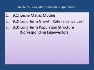
Introduction to Leslie Models. Pierre Auger IRD UR Geodes, Centre de recherche de l’Ile de France, Bondy et Ecole Normale Supérieure de Lyon. AIMS 24/01/06. Population matrix models H. Caswell. 1. 2. i. w. âge( x ). …. i -1. i. w. 0. 1. 2. Structured populations. Structured :

Introduction to Leslie Models
E N D
Presentation Transcript
Introduction to Leslie Models Pierre Auger IRD UR Geodes, Centre de recherche de l’Ile de France, Bondy et Ecole Normale Supérieure de Lyon AIMS 24/01/06
Population matrix models H. Caswell
1 2 i w âge(x) … i -1 i w 0 1 2 Structured populations • Structured : • size • Stage • age S. Charles, Lyon 1
Linear models L is a constant non negative matrix (Lij/ 0 for alli,j ) Matrix equations of this type were first used to describe the dynamics of age-structured populations : Bernardelli H., Population waves, Journal of the Burma research Society, 31, 1941. Leslie P.H., on the use of matrices in certain population mathematics, Biometrika 35, 1945.
Structured populations The individuals of a population are categorized in a finite number n of classes (e.g. by age, by size, by weight). • Let ni(t) the number of individuals in the ith class i=1,…,n, at time t=1,2,... • Denote sj the fraction of j-class individuals expected to survive and move to class j+1 per unit of time (0 . sj. 1) • and fi the expected number of offsprings per j-class individual per unit of time (fi/ 0)
Fecundity 1 2 3 … w-1 w Life cycle Survival S1 S2 Sw-1
Leslie model At time t+1: • The number of newborns is : • The number of j-class individuals who survive at time t+1 is :
Leslie matrix Leslie (1948)
Leslie and Usher matrices • Leslie matrix models: Population is divided into age classes, all of which have the same length. The width of the age-classes equals the projection interval. • Usher matrix models: individuals are categorized by size classes. No individual can shrink in size or grow more than one class in one unit of time.
Irreducible matrix Theorem: A matrix is irreducible if an only if its associated graph is strongly connected (contains a path from every node to every other node . If we exclude the post reproductive classes then, most life cycle graphs are strongly connected
Reducible life cycle F3 P4 F2 P1 P2 P3 1 2 3 4
Reducible matrix If L is reducible, then decompose into a block triangular matrix.
Primitive matrix A nonnegative irreducible matrix L is primitive if Lk > 0 for some integer k. Theorem A non negative irreducible matrix L is primitive if and only if the greatest common divisor of the lengths of the loops of its graph is equal to one. If L is non primitive, the gcd of the loops of the graph d>1 is the index of imprimitivity, it means that there is an inherent cyclicity in the life cycle
Imprimitive life cycle : d=4 F4 P1 P2 P3 1 2 3 4
Primitive life cycle F3 F2 P1 P2 1 2 3
Frobenius theorem Theorem :A non negative irreducible primitive matrix L has a positive real eigenvalue which is a simple root of the characteristic equation V1 (V1/ rVir for any other eigenvalue Viof L) and to this eigenvalue there corresponds a positive right eigenvector (U > 0, LU = V1 U ) and a positive left eigenvector (V > 0, VT L = V1 VT ).
1 2 3 … w-1 w Perron-Frobenius theorem A is primitive
Strong ergodic theorem Asymptotic growth rate Asymptotic age-class distribution
Bilan démographique Modèle déterministe: l = 0,96
Perron-Frobenius theorem Theorem : If L is irreducible but imprimitive (cyclic) with index of imprimitivity d, there exists a simple strictly dominant eigenvalue V1 (rV1r/ rVir for any other eigenvalue Vi of L) and to this eigenvalue there correspond positive right and left eigenvectors. But, there are d-1 complex eigenvalues V equal in magnitude to V1 such as: V=V1 exp(2kpi/d).
Structured populations The problem can be : • Linear autonomous if A is constant. • Linear nonautonomous if A depends explicitly on time t (A=A(t)). • Nonlinear if A = A(t,n(t)).
Effect of landscape fragmentation on an insect population dynamics(Abax parallelepipedus: Coleoptera, Carabidae) Pierre Auger*, Françoise Burel**, Jean-Baptiste Pichancourt***IRD UR Geodes, Centre de recherche de l’Ile de France, Bondy et Ecole Normale Supérieure de Lyon, Institut des Systèmes Complexes.**ECOBIO, CNRS, Université de Rennes 1
L’alouette des champs est l’une des espèces des paysages agricoles dont les effectifs ont été les plus affectés par les pratiques agricoles. Courtesy of English Nature In Europe, more than 50% of lands are cultivated Increasing industrial agriculture and reduction of semi-natural habitats Loss of biodiversity « La conservation de la biodiversité sur ces espaces agricoles est devenue aussi préoccupante que dans les espaces semi-naturels ou protégés ». Krebs et al. « The second silent spring », Nature 1999,
Changes of landscape structure Increasing intensive agriculture 1974 2000 Decreasing the proportion of semi-natural habitats Increasing the proportion of intensively cultivated surfaces Increase of pesticides and fertilizers
Comment assurer la durabilité des paysages de bocage? Ouverture du paysage Quel est le seuil maximal d’ouverture du paysage au delà duquel les populations déclinent? quel est le linéaire minimal de haies, nécessaires au maintien des espèces caractéristiques du bocage ?
How to manage the landscape ? • Mathematical modelling : a tool for predicting effects of management • Coupling physical and population models
A Model for population dynamics of an insect in a heterogeneous environment
woodlot Intersection Linear element Populations Individual fluxes Target species: Abax parallelepipedus Walking species Mainly found in woods Also in hedges and « Bocage » Can be found in lanes Presence depends on: Hedge connectivity Wood areas Existence of lanes
H Leslie Matrix Model Diffusion Matrix (stepping stone) Goes away from M B, CC ou H Remains in B Few differences between B and CC L A1 A2 F13 S21 S32 S33 A. Spatial Leslie model Wood (B) « Bois » B Lanes (CC) « Chemin Creux » CC Hedges (H) M Agricultural Matrix (M) : Maïs Fécondity (f) : f(B) et f(CC) Survival (s): s(B)=s(CC) > s(H) > s(M)
% B M H CC Implicit model of landscape B. Landscape model and diffusion Landscape (network) Transition coefficients (qij) Diffusion model mij = pj . qij Martin (2001); Pichancourt et al. (unpublished)
k increases Fragmentation = decreasing the amount of favorable elements (example : wood) + evolution from large to small patches
Agreggation of variables The complete model AGGREGATION k>>1 Aggregated vector Aggregated Model Leslie Model Asymptotic growth rate l Asymptotic age class distribution
B M CC Using the complete model Using the aggregated model Agreggation of variables (10% CC)
B M M M M H CC CC B B H B Studying different cases • Wood and matrix • Effect of lanes: CC = 5% • Effect of hedges: H = 5 % • Effect of lanes and hedges:CC = 5 %, H = 5 %
Looking for : • Asymptotic growth rate () • Asymptotic age class distribution ( ) • Asymptotic spatial distribution ( )
Effect of lanes and hedges on B B M M B M 5 % CC CC CC H H Fragmentation k % B 5 % H + 5 % CC B M 5 % H k
% Adultes % Larves B M Asymptotic age class distribution
Interprétations • Woods • = Target patches to be maintained to reduce fragmentation. • Lanes • = Have a positive effect on population viability. • Hedges • = Have a negative effect on population viability for a rather small level of fragmentation (sink effect) also shown by (Martin 2000, Tischendorf et al. 1998)
Conclusion : Evaluate biodiversity loss according to various management programs Define public policies Propose management programs
Perspectives • Non linear models • Effects of pesticides • Predation • Spatially explicit modelling