The Theory for Gradient Chromatography Revisited
200 likes | 405 Vues
by Jan Ståhlberg Academy of Chromatography www.academyofchromatography.com. The Theory for Gradient Chromatography Revisited. Objective of the presentation. Discuss the background of the traditional theory for gradient chromatography.

The Theory for Gradient Chromatography Revisited
E N D
Presentation Transcript
by Jan Ståhlberg Academy of Chromatography www.academyofchromatography.com The Theory for Gradient Chromatography Revisited
(c) Academy of Chromatography 2007 Objective of the presentation Discuss the background of the traditional theory for gradient chromatography. Show how a more fundamental and general theory for gradient chromatography can be obtained. Show some applications of the general theory.
Brief review of the traditional theory (1) The traditional derivation starts with the velocity of the migrating zone as a function of the local retention factor. us Mobile phase velocity F(x,t) Zone velocity Local retention factor as a function of mobile phase composition F
Brief review of the traditional theory (2) Introduce the coordinate z where: Assume that a given composition of the mobile phase migrates through the column with the same velocity as the mobile phase, i.e. u0. Let the solute be injected at x=0 and t=0. The equation for the migrating zone can now be written:
Brief review of the traditional theory (3) The retention time is found from the integral: In many cases the retention factor of a solute decreases exponentially with F, i.e.: Where S is a constant characteristic of the solute.
Brief discussion of the traditional theory (4) • For a linear gradient with slope G and for a solute with retention factor ki at t=0, integration gives:
Mass balance approach(1) A fundamental starting point for an alternative gradient theory is the mass balance equation for chromatography: c= solute concentration in the mobile phase n= solute concentration on the stationary phase F= column phase ratio D= diffusion coefficient of the solute x= axial column coordinate t= time
Mass balance approach(2) The stationary phase concentration is a function of the mobile phase composition, Φ, i.e. n=n(c,Ф(x,t)) . This means that: For a linear adsorption isotherm F*δn/ δ c is equal to the retention factor k(Ф(x,t)).
Mass balance approach(3) The mass balance equation becomes:. Here, the diffusive term has been omitted. The equation is the analogue of the ideal model for chromatography. The term ∂n/∂Φ is a function of c, i.e. In the limit c→0, the traditional representation of gradient chromatography theory is obtained.
Mass balance approach(4) For a solute it is often found that: Where c is the concentration of the solute in the mobile phase and k0 the retention factor of the solute when Ф =0. The function ∂Ф/∂t is known and determined by the experimenter. For a linear gradient it is equal to the slope, G, of the gradient.
Mass balance approach(5) For this particular case the mass balance equation is: Where ki is the initial retention factor at t=0. The solution of this equation is of the form: where f(x,t) is determined by the boundary and initial conditions.
Mass balance approach(6) Example: Assume that the solute is injected at x=0 as a Gaussian profile according to The solution of the differential equation is found to be:
Solution of the gradient equation for a Gaussian profile, red line. Numeric simulation of the complete mass balance equation, H=10mm, for the same input parameters. c0=10 mmol, t0=50,s ki=10, ,ti=10s Gradient equation; Gaussian injection;S*G=5
Solution of the gradient equation for a Gaussian profile, red line. Numeric simulation of the complete mass balance equation, H=10mm, for the same input parameters. c0=10mmol, t0=50,s ki=10, ,ti=10s Gradient equation; Gaussian injection;S*G=1
Solution of the gradient equation for a Gaussian profile, red line. Numeric simulation of the complete mass balance equation, H=10mm, for the same input parameters. c0=10 mmol, t0=50,s ki=10, ,ti=10s Gradient equation; Gaussian injection;S*G=0.1
Solution of the gradient equation for a Gaussian profile, red line. Numeric simulation of the complete mass balance equation, H=10mm, for the same input parameters. c0=10 mmol, t0=50,s ki=10, ,ti=10s Gradien equation; Gaussian injection;S*G=0.05
Solution of the gradient equation for a Gaussian profile, red line. Numeric simulation of the complete mass balance equation, H=10mm, for the same input parameters. c0=10 mmol , t0=50,s ki=10, ,ti=10s Gradient equation; Gaussian injection: S*G=0.01
Mass balance approach(7) Example: Assume that the solute is injected at x=0 as a profile according to The solution of the differential equation is:
Mass balance approach(8) Example: Assume that the solute concentration is constant and independent of time. The solution of the differential equation is:
Conclusions • A fundamental and general theory for gradient chromatography can be obtained from the mass balance equation for chromatography. • The traditional theory for gradient chromatography is a special case of a more general theory, it is valid in the limit c(solute) 0. • By neglecting the dispersive term in the mass balance equation, algebraic solutions are easily found. • Practical consequences: • By comparing experimental data with the exact solution, the effect of dispersion can be quantified. • ……..