Variational Formulation
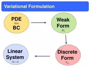
Variational Formulation. PDE With BC. Weak Form. Linear System. Discrete Form. Variational Formulation. PDE With BC. Weak Form. where. Variational Formulation. BVP. Weak Formulation ( variational formulation).

Variational Formulation
E N D
Presentation Transcript
Variational Formulation PDE With BC Weak Form Linear System Discrete Form
Variational Formulation PDE With BC Weak Form where
Variational Formulation BVP Weak Formulation ( variational formulation) Multiply equation (1) by and then integrate over the domain Green’s theorem gives where
Triangulation We have We have
Weak Formulation ( variational formulation) Infinite dimensional space Finite dim subspace Space of all cont. pcw-linear
Discrete Form Linear System approximate u In expanded form In Matrix form This is a linear system of 5 equations in 5 unknowns
The approximate Solution Once this linear system is solved we obtain an approximation to the solution In Matrix form Remark: Remark: We are going to focus our attention in the efficient construction of this stiffness matrix
Sparsity In Matrix form Remark: This matrix is sparse (many zeros) few non-zero entries another example
Sparsity Sparsity of the matrix # of nonzero =1153 312 triangles and 177nodes Use spy(A) to see sparsity
Local basis function and global basis function 5 12 13 Global basis function If we restrict the function to the triangle K12 it becomes one of the local basis functions for K12 K12 has 3 local basis functions Matrix t
Remark: This matrix is sparse (many zeros) few non-zero entries Assembly of the Stiffness Matrix Remark: These few nonzero entries are computed by looping over all triangles In Matrix form Remark: nonzero entry is a sum of integrals of local basis functions over a triangle
Assembly of the Stiffness Matrix Step1 primary stiffnes matrix Loop over all triangles 1 -16. in each triangle, we calculate 3x3 matrix which involves calculating 9 integrals of all possible combination of local basis functions. Step2 impose boundary condition After we assemble the primary stiffness matrix in step1, we enforce the boundary condition by forcing the corresponding coefficient to be zero.
Step1 primary stiffnes matrix For k = 1 : 16 Step1a: find all gradients Step1b: Find 9 integrals Step1c: Add these contributions to the primary stiffness matrix End the loop
Find the gradients with cyclic permutation of the index i,j k over 1,2,3
Find the gradients with cyclic permutation of the index i,j k over 1,2,3 function [area,b,c] = Gradients(x,y) area=polyarea(x,y); b=[y(2)-y(3); y(3)-y(1); y(1)-y(2)]/2/area; c=[x(3)-x(2); x(1)-x(3); x(2)-x(1)]/2/area;
Step1 primary stiffnes matrix Loop over all triangles 1 -16 for example K9 10 5 13
Step1 primary stiffnes matrix We want to compute: local basis functions Find gradient for each Find 3x3 matrix Loop over all triangles 1 -16. for example K9 10 5 13
Step1 primary stiffnes matrix We want to compute: local basis functions Find gradient for each Find 3x3 matrix Loop over all triangles 1 -16. for example K9 10 5 13
Step1 primary stiffnes matrix We want to compute: local basis functions Find gradient for each Find 3x3 matrix Loop over all triangles 1 -16. for example K9 10 5 13
Step1 primary stiffnes matrix We want to compute: local basis functions Find gradient for each 10 5 13 Find 3x3 matrix Local to global
Step1 primary stiffnes matrix We want to compute: local basis functions Find gradient for each 10 5 13 Find 3x3 matrix Local to global
Step1 primary stiffnes matrix Triangle K10 1 2 3 1 1 -1/2 -1/2 2 -1/2 1/2 0 3 -1/2 0 1/2 Local to global 5 10 11 5 1 -1/2 -1/2 10 -1/2 1/2 0 11 -1/2 0 1/2
K =1 1/2 0 -1/2 0 1/2 -1/2 -1/2 -1/2 1 K =2 1/2 0 -1/2 0 1/2 -1/2 -1/2 -1/2 1 K = 3 1/2 0 -1/2 0 1/2 -1/2 -1/2 -1/2 1 K =4 1/2 0 -1/2 0 1/2 -1/2 -1/2 -1/2 1 K =13 1/2 0 -1/2 0 1/2 -1/2 -1/2 -1/2 1 K =14 1/2 0 -1/2 0 1/2 -1/2 -1/2 -1/2 1 K =15 1/2 0 -1/2 0 1/2 -1/2 -1/2 -1/2 1 K =16 1/2 0 -1/2 0 1/2 -1/2 -1/2 -1/2 1
Step1 primary stiffnes matrix 1 0 0 0 0 0 0 1 0 0 0 0 0 0 1 0 0 0 0 0 0 1 0 0 0 0 0 0 4 0 0 0 0 0 0 2 0 0 0 0 0 0 0 0 0 0 0 0 0 0 0 0 0 0 -1 0 0 0 -1 -1 0 -1 0 0 -1 -1 0 0 -1 0 -1 0 0 0 0 -1 -1 0 0 0 0 -1 0 0 0 0 0 0 0 -1 0 0 0 0 0 0 0 -1 0 0 0 0 0 0 0 -1 0 0 0 -1 -1 -1 -1 0 0 0 -1 -1 0 0 2 0 0 0 -1 -1 0 0 2 0 0 0 -1 -1 0 0 2 -1 0 0 -1 0 0 -1 4 0 0 0 -1 0 0 0 4 0 0 -1 -1 0 0 0 4 0 0 -1 -1 0 0 0 4 function A = StiffMat2D(p,t) np = size(p,2); nt = size(t,2); A = sparse(np,np); for K = 1:nt loc2glb = t(1:3,K); % local-to-global map x = p(1,loc2glb); % node x-coordinates y = p(2,loc2glb); % node y- [area,b,c] = Gradients(x,y); AK = (b*b'+c*c')*area; % element stiff mat A(loc2glb,loc2glb) = A(loc2glb,loc2glb)+ AK; % add element stiffnesses to A end
Assemble the Load vector L In Matrix form
Assembly of the Load Vector Step1 primary Load vector Loop over all triangles 1 -16. in each triangle, we calculate 3x1 matrix which involves calculating 3 integrals Step2 impose boundary condition After we assemble the primary load vector and stiffness matrix in step1, we enforce the boundary condition by forcing the corresponding coefficient to be zero.
The load vector b is assembled using the same technique as the primary stiffness matrix A, that is, by summing element load vectors BKover the mesh. On each element K we get a local 3×1 element load vector BKwith entries BKi = ∫Kf φi dx; i = 1;2;3 Using node quadrature, we compute these integrals we end up with BKi≈ 1/3f (Ni)|K|; i = 1;2;3 We summarize the computation of the load vector with the following Matlab code.
function b = LoadVec2D(p,t,f) np = size(p,2); nt = size(t,2); b = zeros(n,1); for K = 1:nt loc2glb = t(1:3,K); x = p(1,loc2glb); y = p(2,loc2glb); area = polyarea(x,y); bK = [f(x(1),y(1)); f(x(2),y(2)); f(x(3),y(3))]/3*area; % element load vector b(loc2glb) = b(loc2glb) ... + bK; % add element loads to b end