
Incremental Methods for Machine Learning Problems
E N D
Presentation Transcript
Incremental Methods for Machine Learning Problems Aristidis Likas Department of Computer Science University of Ioannina e-mail: arly@cs.uoi.gr http://www.cs.uoi.gr/~arly
Outline Machine Learning: Data Modeling + Optimization The incremental machine learning framework Global k-means (PR, IEEE TNN) Greedy EM (NPL 2002, Bioinformatics) Incremental Bayesian GMM learning (IEEE TNN) Dip-Means Incremental Bayesian Supervised learning (IEEE TNN) Current research problems Matlab code available for all methods
Machine Learning Problems Unsupervised Learning Clustering Density estimation Dimensionality Reduction Supervised Learning Classification Regression Also considered as Data mining or Pattern Recognition problems
Machine Learning as Optimization To solve a machine learning problem • dataset X of training examples • parametric Data Model that ‘explains’ the data • f(x;Θ), Θset of parameters to be estimated during training • objective function L(X;Θ) Model training is achieved through the optimization of the objective function. • Usually non-convex optimization, many local optima • We search for a ‘near-optimal’ solution
Machine Learning as Optimization • Local search algorithms (gradient descent, BFGS, EM, k-means) • Performance depends on the initialization of parameters. • Typical solution: multiple (random) restarts • multiple local search runs from (random) initializations • Keep the solution of the best run • Weakenesses: • poor solutions for large models • How many runs? • How to initialize? • non-determinism: non-repeatability, difficulty in comparing different methods. • An alternative approach (in some cases): • incremental model training
Building Blocks formulation • Many popular Data Models can be written as a combination (or simply as a set) of “Building Blocks” • Number of BBs = model order • The combination function may also include parameters (w1,…, wM) • Set of model parameters: • Examples • k-means Clustering: Β=cluster centers, L=clustering error • Mixture Models: B=component densities, L=Likelihood • FF Neural Networks: B=sigmoidal or RBF hidden units, L=LS error • Kernel Models: B=basis functions (kernels) , L=loss functions
Building Blocks • In some models building blocks are fixeda priori. • Only optimization w.r.t to the combination weights wi is required (convex problem in many cases, eg SVM). • In the general case all the BB parameters θi should be learnt. • Non-convex optimization problem • many local optima • local search methods • dependence on initialization of ΘM • Resort to incremental training
Incremental training • The incremental (greedy) approach can offer a simple and effective solution to the random restarts problem in training ML models. • Incremental methods are based on the following assumption: • We can obtain a ‘near-optimal’ model with k BBs by exploiting a ‘near-optimal’ model with (k-1) BBs. • Method: Starting with k=1 BB, incremental methods sequentially add one BB at each step until M BBs have been added.
Incremental Training Approaches • 1. Fast approach: optimize only wrt θk of the k-ΒΒ keeping θ1…θk-1 fixed to the solution of (k-1)-BB model. • Exhaustive Enumeration (deterministic) • Multiple restarts, but the search space is much smaller • 2. Fast approach followed by full model training (once) LS
Incremental Training • 3. Full model training with multiple restarts: • Initializations based on the (k-1)-BB model. • Deterministic search is preferable (avoid randomness) • Incremental methods also offer solutions for all indermediate models with k=1,…,M BBs LS LS LS
Prototype-Based Clustering • Partition a dataset X of N vectors xi into M subsets (clusters) Ck such that intra-cluster variance is minimized. • Intra-cluster variance: avg. distance from the cluster prototypemk • k-means: Prototype = cluster center • Finds local minima w.r.t. clustering error • sum of intra-cluster variances • Highly dependent on the initial positions of the centers mk
Global k-means • Incremental, deterministic clustering algorithm that runs k-Means several times • Finds near-optimal solutions wrt clustering error • Idea: a near-optimal solution for k clusters can be obtained by running k-means from an initial state • the k-1 centers are initialized from a near-optimal solution of the (k-1)-clustering problem • the k-th center is initialized at some data point xn (which?) • Consider all possible initializations (one for each xn)
Global k-means • In order to solve the M-clustering problem: • Solve the 1-clustering problem (trivial) • Solve the k-clustering problem using the solution of the (k-1)-clustering problem • Execute k-Means N times, initialized as at the n-th run (n=1,…,N). • Keep the solution corresponding to the run with the lowest clustering error as the solution with k clusters • k:=k+1, Repeat step 2 until k=M.
Best Initial m2 Best Initial m3 Best Initial m4 Best Initial m5
Fast Global k-Means • How is the complexity reduced? • We select the initial state that provides the greatest reduction in clustering error in the first iteration of k-means (reduction can be computed analytically) • k-means is executed only once from this state
Kernel-Based Clustering(non-linear separation) • Given a set of objects and the kernel matrix K=[Kij] containing the similarities between each pair of objects • Goal: Partition the dataset into subsets (clusters) Ck such that intra-cluster similarity is maximized. • Kernel trick: Data points are mapped from input space to a higher dimensional feature spacethrough a transformationφ(x). • The kernel function corresponds to the inner product in feature space • Kernel k-Means ≡ k-Means in feature space
Kernel k-Means • Kernel k-means = k-means in feature space • Minimizes the clustering error in feature space • Differences from k-means • Cluster centers mk in feature space cannot be computed • Each cluster Ck is explicitly described by its data objects • Computation of distances from centers in feature space: • Finds local minima - Strong dependence on the initial partition
Global Kernel k-Means • In order to solve the M-clustering problem: • Solve the 1-clustering problem with Kernel k-Means (trivial solution) • Solve the k-clustering problem using the solution of the (k-1)-clustering problem • Let denote the solution to the (k-1)-clustering problem • Execute Kernel k-Means N times, initialized during the n-th run as • Keep the run with the lowest clustering error as the solution with k clusters • k := k+1 • Repeat step 2 until k=M. • The fast Global kernel k-means can be applied
Best Initial C2 Best Initial C3 Empty circles: optimal initialization of the cluster to be added Best Initial C4
Global Kernel k-means - Applications • MRI image segmentation • Key frame extraction - shot clustering
Mixture Models • Probability density estimation: estimate the density function model f(x) that generated a given dataset X={x1,…, xN} • Mixture Models • M pdf componentsφj(x), • mixing weights: π1, π2, …, πM (priors) • Gaussian Mixture Model (GMM): φj = N(μj, Σj)
GMM (graphical model) πj Hidden variable observation
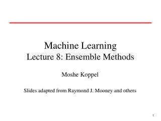
GMM examples GMMs be used for density estimation (like histograms) or clustering Cluster memberhsip probability
Mixture Model training Givena dataset X={x1,…, xN} and a GMM f (x;Θ) Likelihood: GMM training: log-likelihood maximization Expectation-maximization (EM) algorithm Applicable when posterior P(Z|X) can be computed
EM for Mixture Models • E-step: compute expectation of hidden variables given the observations: • M-step: maximize expected complete likelihood
EM for GMM (M-step) Mean Covariance Mixing weights
Greedy EM for GMM • Start with k=1, f1(x)=N(μ1, Σ1), μ1=mean(X), Σ1=cov(X) • Let fk the GMM solution with k components • Let φ(x;μ,Σ) the k+1 component to be added • Refinefk+1(x) using EM -> final GMM with k+1 components
Greedy EM for GMM • Σ=σΙ, • Given θ=(μ,σ), α* can be computed analytically - Remark: the new component should be placed in a data region - Deterministic approach
Greedy-EM applications • Image modeling for content-based retrieval and relevance feedback • Motif discovery in sequences (discrete data, mixture of multinomials) • Times series clustering (mixture of regression models)
Bayesian GMM Typical approach: Priors on all GMM parameters
Bayesian GMM training • Parameters Θ become (hidden) RVs: H={Z, Θ} • Objective: Compute Posteriors P(Z|X), P(Θ|X) (intractable) • Approximations • Sampling (RJMCMC) • MAP approach • Variational approach • MAP approximation • mode of the posterior P(Θ|Χ) (MAP-EM) • compute P(Z|X,ΘMAP)
Variational Inference (no parameters) • Computes approximation q(H) of the true posterior P(H|X) • For any pdf q(H): • Variational Bound(F) maximization • Mean field approximation • System of equations
Variational Inference (with parameters) • X data, H hidden RVs, Θ parameters • For any pdf q(H;Θ): • Maximization of Variational BoundF • Variational EM • VE-Step: • VM-Step:
Bayesian GMM training • Bayesian GMMs • mean field variational approximation • tackles the covariance singularity problem • requires to specify the parameters of the priors • Estimating the number of components: • Start with a large number of components • Let the training process prune redundant components (πj=0) • Dirichlet prior on πjprevents component prunning
Bayesian GMM without prior on π • Mixing weights πjare parameters (remove Dirichlet prior) • Training usingVariational EM • Method (C-B) • Start with a large number of components • Perform variational maximization of the marginal likelihood • Prunning of redundant components (πj=0) • Only components that fit well to the data are finally retained
Bayesian GMM (C-B) • C-B method: Results depend on • the number of initial components • initialization of components • specification of the scale matrix V of the Wishart prior p(T)
Incremental Bayesian GMM • Solution: incremental training using component splitting • Local scale matrix V: based on the variance of the component to be splitted • Modification of the Bayesian GMM is needed • Divide the components as ‘fixed’ or ‘free’ • Prior on the weights of ‘fixed’ components (retained) • No prior on the weights of ‘free’ components(may be eliminated) • Prunning restricted among ‘free’ components
Incremental Bayesian GMM • Start with k=1 component. • At each step: • select a component j • split component j in two subcomponents • set the scale matrix V analogous to Σj • apply Variational EM considering the two subcomponents as free and the rest components as fixed • either the two components will be retained and adjusted • or one of them will be eliminated and the other one will recover the original component (before split) • until all components have been tested for split unsuccessfully
Incremental Bayesian GMM Image segmentation Number of segments determined automatically
Incremental Bayesian GMMImage segmentation Number of segments determined automatically
Relevance Vector Machine • RVM model (Tipping 2001) • φi(x)=K(x,xi) (same kernel function ‘centered’ on training example xi) • Fixed pool of N basis functions • Initially M=N basis functions: • Bayesian inference with sparse prior on w prune redundant basis functions • Οnly few basis functions are retained (relevance vectors)
Relevance Vector Machine • Likelihood: • Sparse prior of w: - Separate precision αi for each weight wi • Weight prior p(w): Student's t (enforces sparsity)
RVM Training • Maximize Marginal Likelihood • Use Expectation Maximization (EM) Algorithm: • E-step: • M-step: • Sparsity: Most
RVM Incremental Training Incrementally add basis functions starting with empty model (Faul & Tipping 2003) Optimization w.r.t a single parameter αi Estimation of optimalαianalytical:
RVM Incremental Training • At each iteration of the training algorithm • Compute optimal αi for all Ν basis functions • Select the bestbasis function φi(x)from the pool of N candidates • Perform one of the following: • Add this basis function to the current model • Update αi (if it is included in the model) • Remove this basis function (if it is included in the model and αi=∞)
RVM Limitations • How to specifykernel parameter? (e.g. scale of RBF kernel) • Typical solution: Cross-validation • Computationally expensive • Cannot be used when many parameters must be adjusted • How to model non-stationary functions? • RVM uses the same kernel for whole input space
Adaptive RVM with Kernel Learning (aRVM) • Assume different parametersθi for each φ(x;θi) • RBF kernel: centermi and scale hi are parameters • Generally mi different from training points xn • Employ incremental RVM training • Typical incremental RVM: select from a fixed set of N basis functions the best basis function to add • aRVM: select the basis function φ(x;θi) to add by optimizing marginal likelihood sl(αi,θi) w.r.t (αi,θi)