Enhancing Downlink MU-MIMO Performance with Interference Cancellation
220 likes | 251 Vues
Explore how interference cancellation boosts DL MU-MIMO, minimizing errors in CSI feedback. Learn about MMSE processing, sources of CSI errors, simulation results, and the impact of feedback delay errors. Gain insights into the performance of MU-MIMO with IC across various feedback error levels.

Enhancing Downlink MU-MIMO Performance with Interference Cancellation
E N D
Presentation Transcript
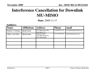
Interference Cancellation for Downlink MU-MIMO Date: 2009-11-17 Authors: Sameer Vermani, Qualcomm
Abstract • MU-MIMO provides significant performance gains over single user Tx BF for reasonable product configurations • Interference Cancellation (IC) makes downlink (DL) MU-MIMO more robust • To support Interference Cancellation in DL MU-MIMO: • Each client should receive as many LTFs as needed to train the total number of spatial streams in the DL • Each client should know which spatial streams are meant for it Sameer Vermani, Qualcomm
Outline Introduction Interference Cancellation Receive processing Sources of CSI Error at AP Simulation results for 40MHz and reasonable product configurations AP 4TX; Clients are 1x2 AP 8TX; Clients are 1x2 Conclusions Sameer Vermani, Qualcomm
Introduction to Interference Cancellation • In DL MU-MIMO, clients can have more receive (Rx) antennas than the number of spatial streams they receive • The additional antennas can be used for Interference Cancellation (IC) / Interference Suppression • Particularly useful when precoding is imperfect due to errors in the CSI available at the AP • This calls for a DL MU-MIMO preamble design that can support IC • Each client should receive as many LTFs as needed to train the total number of spatial streams in the DL • Each client should know which spatial streams are meant for it Sameer Vermani, Qualcomm
Receive MMSE for Interference Suppression • For instance, consider a 4-antenna AP transmitting 1 ss each to 4 STAs each with 2 Rx antennas, the Rx signal at 8 Rx antennas is given by: • The equivalent precoded channel is Hequiv = H8x4W4x4 • The first two rows of Hequiv is the channel seen by STA1; H1 = Hequiv(1:2,:) • STA1 can do the following MMSE processing to reduce the interference from other STAs: where the first element of x1 gives the estimate of the symbol for STA1 and 12is the noise variance at STA1 Sameer Vermani, Qualcomm
Sources of CSI Errors at AP • Pathloss to the STA or the amount of quantization in the CSI feedback report • The channel estimation SNR or quantization level is fundamental to the accuracy of CSI • Time variations in the channel • A non-zero time interval between DL MU-MIMO transmission and CSI feedback causes discrepancies between the actual channel and precoding weights • Feedback delay of 10 ms results in an error floor of -25 dBc (assuming a coherence time of 400 ms) • Modeled as two independent additive noise sources in the CSI • CSI Feedback Delay Error Floor {-20, -25, -30} dBc • Channel Estimation Error Floor (Pathloss dependent) • At high SNRs, CSI feedback error will dominate and at low SNRs pathloss errors will dominate. Sameer Vermani, Qualcomm
Simulations • Determine the gains of using MU-MIMO and Interference Cancellation (IC) • We plot the 10 percentile and 50 percentile points from the CDF of the aggregate PHY throughput (measured at the AP) as a function of pathloss • For comparison, we also plot the corresponding sequential beamforming (BF) data quantities • SVD based transmission with equal MCS per spatial stream • Data rates averaged across sequential transmissions to the clients Sameer Vermani, Qualcomm
Results for 4 antenna AP, Four 1x2 clients, full loading Sameer Vermani, Qualcomm
Simulation Parameters • AP with 4 Tx antennas transmitting at 24 dBm • Noise floor of -89.9 dBm • 4 STA with 2 Rx antenna each • -35 dBc of TX distortion • Equal Pathloss to each STA, varied from 70 to 95 dB • Single SS per STA in the MU-MIMO case and 2 ss for Tx BF case • TGac Channel Model D, NLOS • Results for 200 channel realizations • For MU-MIMO, MMSE precoding done to beam-form the 1 ss of each STA to one of its antennas • Two sources of CSI error at AP • Channel estimation floor at client = -(Total Tx Power – Pathloss + 89.9 dBm (Thermal noise)) • Feedback delay error = {-20, -25 ,-30} dBc Sameer Vermani, Qualcomm
Eigen BF TDMA MU-MIMO w/o IC MU-MIMO with IC Eigen BF TDMA MU-MIMO w/o IC MU-MIMO with IC 4 antenna AP, Four 1x2 clients, -20 dBc feedback error • MU-MIMO with IC gives best performance • Interference Cancellation improves performance for a poor CSI accuracy • IC enables full loading • Compare with slide 21 in Appendix, which shows the 3 ss results • Performance better with 3 ss in the absence of IC Sameer Vermani, Qualcomm
Eigen BF TDMA MU-MIMO w/o IC MU-MIMO with IC Eigen BF TDMA MU-MIMO w/o IC MU-MIMO with IC 4 antenna AP, Four 1x2 clients, -25 dBc feedback error • For all pathlosses between 70 and 95, MU-MIMO with IC gives substantial gains Sameer Vermani, Qualcomm
Eigen BF TDMA MU-MIMO w/o IC MU-MIMO with IC Eigen BF TDMA MU-MIMO w/o IC MU-MIMO with IC 4 antenna AP, Four 1x2 clients, -30 dBc feedback error • For all pathlosses between 70 and 95, MU-MIMO with IC gives best performance • Gains of IC reduce as CSI accuracy improves Sameer Vermani, Qualcomm
Results for 8 antenna AP, Six 1x2 clients Sameer Vermani, Qualcomm
Simulation Parameters • AP with 8 Tx antennas transmitting at 24 dBm • Noise floor of -89.9 dBm • 6 STA with 2 Rx antenna each • -35 dBc of TX distortion • Equal Pathloss to each STA, varied from 70 to 95 dB • Single SS per STA in the MU-MIMO case and 2 ss for Tx BF case • TGac Channel Model D, NLOS • Results for 200 channel realizations • For MU-MIMO, MMSE precoding done to beam-form the 1 ss of each STA to one of its antennas • Two sources of CSI error at AP • Channel estimation floor at client = -(Total Tx Power – Pathloss + 89.9 dBm (Thermal noise)) • Feedback delay error = {-20, -25 ,-30} dBc Sameer Vermani, Qualcomm
Eigen BF TDMA MU-MIMO w/o IC MU-MIMO with IC Eigen BF TDMA MU-MIMO w/o IC MU-MIMO with IC 8 antenna AP, Six 1x2 clients, -20 dBc feedback error • MU-MIMO with IC gives best performance • IC improves performance for a poor CSI accuracy Sameer Vermani, Qualcomm
Eigen BF TDMA MU-MIMO w/o IC MU-MIMO with IC Eigen BF TDMA MU-MIMO w/o IC MU-MIMO with IC 8 antenna AP, Six 1x2 clients, -25 dBc feedback error • For all pathlosses between 70 and 95, MU-MIMO with IC gives best performance Sameer Vermani, Qualcomm
Eigen BF TDMA MU-MIMO w/o IC MU-MIMO with IC Eigen BF TDMA MU-MIMO w/o IC MU-MIMO with IC 8 antenna AP, Six 1x2 clients, -30 dBc feedback error • Gains of IC reduce here • Precoding is very good Sameer Vermani, Qualcomm
Conclusions • Performance gains for MU-MIMO are huge when compared to single user Tx BF • For reasonable product configurations and wide range of pathlosses • IC makes MU-MIMO robust to poor CSI accuracy at the AP • Dependent on the CSI errors at the AP, IC helps enable fully loaded MU-MIMO • This calls for a DL MU-MIMO preamble design that can support IC • Each client should receive as many LTFs as needed to train the total number of spatial streams in the DL • Each client should know which spatial streams are meant for it Sameer Vermani, Qualcomm
Appendix Data rate calculation Sameer Vermani, Qualcomm
Methodology used to get to Data Rate CDFs • For each spatial stream • Calculate the post processing SINR on each tone • Map the post processing SINR to capacity using log(1+SINR) • Average the capacity across tones to get Cav • Use Cav to calculate SINReff using Cav = log(1+ SINReff) • Map the SINReff to a rate using the AWGN rate table • This method is used in other WAN standards, e.g., 3GPP2 • Sum the rate across all spatial streams for one channel realization to get to aggregate PHY throughput • Do this for 200 channels to get to the CDF of aggregate PHY throughput Sameer Vermani, Qualcomm
Variation of 10 percentile PHY Rates with pathloss Variation of 50 percentile PHY Rates with pathloss Eigen BF TDMA Eigen BF TDMA 800 800 MU-MIMO w/o IC MU-MIMO w/o IC MU-MIMO with IC MU-MIMO with IC 700 700 600 600 500 500 PHY Rate in Mbps measured at AP PHY Rate in Mbps measured at AP 400 400 300 300 200 200 100 100 70 75 80 85 90 95 70 75 80 85 90 95 Pathloss in dB Pathloss in dB 4 antenna AP, Three 1x1 clients, -20 dB feedback error • For all pathlosses between 70 and 95, MU-MIMO gives substantial gains • IC curve lies on top of MU-MIMO w/o IC • In absence of IC, 4 SS MU-MIMO performs worse than 3 SS MU-MIMO • Compare green curve of this slide with blue curve of slide 10 • Better to transmit at 75% loading in the absence of extra antenna at the STAs • Scheduler decision