Too good to be true? The Dream of Arbitrage
Too good to be true? The Dream of Arbitrage. Aswath Damodaran. The Essence of Arbitrage. In pure arbitrage, you invest no money, take no risk and walk away with sure profits. You can categorize arbitrage in the real world into three groups:

Too good to be true? The Dream of Arbitrage
E N D
Presentation Transcript
Too good to be true?The Dream of Arbitrage Aswath Damodaran
The Essence of Arbitrage • In pure arbitrage, you invest no money, take no risk and walk away with sure profits. • You can categorize arbitrage in the real world into three groups: • Pure arbitrage, where, in fact, you risk nothing and earn more than the riskless rate. • Near arbitrage, where you have assets that have identical or almost identical cash flows, trading at different prices, but there is no guarantee that the prices will converge and there exist significant constraints on the investors forcing convergence. • Speculative arbitrage, which may not really be arbitrage in the first place. Here, investors take advantage of what they see as mispriced and similar (though not identical) assets, buying the cheaper one and selling the more expensive one.
Pure Arbitrage • For pure arbitrage, you have two assets with identical cashflows and different market prices makes pure arbitrage difficult to find in financial markets. • There are two reasons why pure arbitrage will be rare: • Identical assets are not common in the real world, especially if you are an equity investor. • Assuming two identical assets exist, you have to wonder why financial markets would allow pricing differences to persist. • If in addition, we add the constraint that there is a point in time where the market prices converge, it is not surprising that pure arbitrage is most likely to occur with derivative assets – options and futures and in fixed income markets, especially with default-free government bonds.
Futures Arbitrage • A futures contract is a contract to buy (and sell) a specified asset at a fixed price in a future time period. • The basic arbitrage relationship can be derived fairly easily for futures contracts on any asset, by estimating the cashflows on two strategies that deliver the same end result – the ownership of the asset at a fixed price in the future. • In the first strategy, you buy the futures contract, wait until the end of the contract period and buy the underlying asset at the futures price. • In the second strategy, you borrow the money and buy the underlying asset today and store it for the period of the futures contract. • In both strategies, you end up with the asset at the end of the period and are exposed to no price risk during the period – in the first, because you have locked in the futures price and in the second because you bought the asset at the start of the period. Consequently, you should expect the cost of setting up the two strategies to exactly the same.
a. Storable Commodities • Strategy 1: Buy the futures contract. Take delivery at expiration. Pay $F. • Strategy 2: Borrow the spot price (S) of the commodity and buy the commodity. Pay the additional costs. (a) Interest cost (b) Cost of storage, net of convenience yield = S k t • If the two strategies have the same costs, F*
Assumptions underlying arbitrage • Investors are assumed to borrow and lend at the same rate, which is the riskless rate. • When the futures contract is over priced, it is assumed that the seller of the futures contract (the arbitrageur) can sell short on the commodity and that he can recover, from the owner of the commodity, the storage costs that are saved as a consequence.
Arbitrage with different borrowing rate and non-recovery of storage costs… • Assume, for instance, that the rate of borrowing is rb and the rate of lending is ra, and that short seller cannot recover any of the saved storage costs and has to pay a transactions cost of ts. The futures price will then fall within a bound. • If the futures price falls outside this bound, there is a possibility of arbitrage
b. Stock Index Futures • Strategy 1: Sell short on the stocks in the index for the duration of the index futures contract. Invest the proceeds at the riskless rate. This strategy requires that the owners of the stocks that are sold short be compensated for the dividends they would have received on the stocks. • Strategy 2: Sell the index futures contract. • The Arbitrage: Both strategies require the same initial investment, have the same risk and should provide the same proceeds. Again, if S is the spot price of the index, F is the futures prices, y is the annualized dividend yield on the stock and r is the riskless rate, the arbitrage relationship can be written as follows: F* = S (1 + r - y)t
Assumptions underlying arbitrage • We assume that investors can lend and borrow at the riskless rate. • We ignore transactions costs on both buying stock and selling short on stocks. • We assume that the dividends paid on the stocks in the index are known with certainty at the start of the period.
Modified Arbitrage • Assume that investors can borrow money at rb and lend money at ra • Assume that the transactions costs of buying stock is tc and selling short is ts. The band within which the futures price must stay can be written as: • Arbitrage is possible if the futures price strays outside this band.
c. T. Bond Futures • The valuation of a treasury bond futures contract follows the same lines as the valuation of a stock index future, with the coupons of the treasury bond replacing the dividend yield of the stock index. The theoretical value of a futures contract should be – where, F* = Theoretical futures price for Treasury Bond futures contract S = Spot price of Treasury bond PVC = Present Value of coupons during life of futures contract r = Riskfree interest rate corresponding to futures life t = Life of the futures contract
Two Special Features of T.Bond Futures • The treasury bond futures traded on the Chicago Board of Trade require the delivery of any government bond with a maturity greater than fifteen years, with a no-call feature for at least the first fifteen years. Since bonds of different maturities and coupons will have different prices, the CBOT has a procedure for adjusting the price of the bond for its characteristics. This feature of treasury bond futures, called the delivery option, provides an advantage to the seller of the futures contract. • There is an additional option embedded in treasury bond futures contracts that arises from the fact that the T.Bond futures market closes at 2 p.m., whereas the bonds themselves continue trading until 4 p.m. The seller does not have to notify the clearing house until 8 p.m. about his intention to deliver. If bond prices decline after 2 p.m., the seller can notify the clearing house of his intention to deliver the cheapest bond that day. If not, the seller can wait for the next day. This option is called the wild card option.
d. Currency Futures • To see how spot and futures currency prices are related, note that holding the foreign currency enables the investor to earn the risk-free interest rate (Rf) prevailing in that country while the domestic currency earn the domestic riskfree rate (Rd). Since investors can buy currency at spot rates and assuming that there are no restrictions on investing at the riskfree rate, we can derive the relationship between the spot and futures prices. • Interest rate parity relates the differential between futures and spot prices to interest rates in the domestic and foreign market.
An Arbitrage Example with Currency Futures • Assume that the one-year interest rate in the United States is 2 percent and the one-year interest rate in Switzerland is 1 percent. Furthermore, assume that the spot exchange rate is $1.10 per Swiss Franc. • The one-year futures price, based upon interest rate parity, should be as follows:
Special Features of Futures Markets • The first is the existence of margins. While we assumed, when constructing the arbitrage, that buying and selling futures contracts would create no cashflows at the time of the transaction, you would have to put up a portion of the futures contract price (about 5-10%) as a margin in the real world. To compound the problem, this margin is recomputed every day based upon futures prices that day – this process is called marking to market - and you may be required to come up with more margin if the price moves against you (down, if you are a buyer and up, if you are a seller). If this margin call is not met, your position can be liquidated and you may never to get to see your arbitrage profits. • The second is that the futures exchanges generally impose ‘price movement limits’ on most futures contracts.
Feasibility of Futures Arbitrage • In the commodity futures market, for instance, Garbade and Silber (1983) find little evidence of arbitrage opportunities and their findings are echoed in other studies. In the financial futures markets, there is evidence that indicates that arbitrage is indeed feasible but only to a sub-set of investors. • Note, though, that the returns are small even to these large investors and that arbitrage will not be a reliable source of profits, unless you can establish a competitive advantage on one of three dimensions. • You can try to establish a transactions cost advantage over other investors, which will be difficult to do since you are competing with other large institutional investors. • You may be able to develop an information advantage over other investors by having access to information earlier than others. Again, though much of the information is pricing information and is public. • You may find a quirk in the data or pricing of a particular futures contract before others learn about it.
Options Arbitrage • Options represent rights rather than obligations – calls gives you the right to buy and puts gives you the right to sell. Consequently, a key feature of options is that the losses on an option position are limited to what you paid for the option, if you are a buyer. • Since there is usually an underlying asset that is traded, you can, as with futures contracts, construct positions that essentially are riskfree by combining options with the underlying asset.
1. Exercise Arbitrage • The easiest arbitrage opportunities in the option market exist when options violate simple pricing bounds. No option, for instance, should sell for less than its exercise value. • With a call option: Value of call > Value of Underlying Asset – Strike Price • With a put option: Value of put > Strike Price – Value of Underlying Asset • You can tighten these bounds for call options, if you are willing to create a portfolio of the underlying asset and the option and hold it through the option’s expiration. The bounds then become: • With a call option: Value of call > Value of Underlying Asset – Present value of Strike Price • With a put option: Value of put > Present value of Strike Price – Value of Underlying Asset
2. Pricing Arbitrage (Replication) • A portfolio composed of the underlying asset and the riskless asset could be constructed to have exactly the same cash flows as a call or put option. This portfolio is called the replicating portfolio. • Since the replicating portfolio and the traded option have the same cash flows, they would have to sell at the same price.
Pricing the Option and Arbitrage Possibilities • Borrowing $22.5 and buying 5/7 of a share today will provide the same cash flows as a call with a strike price of $50. The value of the call therefore has to be the same as the cost of creating this position. Value of Call = Cost of replicating position = • If the call traded at less than $13.21, say $ 13.00. You would buy the call for $13.00 and sell the replicating portfolio for $13.21 and claim the difference of $0.21. Since the cashflows on the two positions are identical, you would be exposed to no risk and make a certain profit. • If the call trade for more than $13.21, say $13.50, you would buy the replicating portfolio, sell the call and claim the $0.29 difference. Again, you would not have been exposed to any risk.
3a. Arbitrage Across Options: Put Call Parity • You can create a riskless position by selling the call, buying the put and buying the underlying asset at the same time. • Since this position yields K with certainty, the cost of creating this position must be equal to the present value of K at the riskless rate (K e-rt). S+P-C = K e-rt C - P = S - K e-rt
Does put call parity hold? • A study in 1977 and 1978 of options traded on the CBOE found violations of put-call parity, but the violations were small and persisted only for short periods. • A more recent study by Kamara and Miller of options on the S&P 500 (which are European options) between 1986 and 1989 finds fewer violations of put-call parity and the deviations tend to be small, even when there are violations.
3b. Mispricing across strike prices and maturities • Strike Prices: A call with a lower strike price should never sell for less than a call with a higher strike price, assuming that they both have the same maturity. If it did, you could buy the lower strike price call and sell the higher strike price call, and lock in a riskless profit. Similarly, a put with a lower strike price should never sell for more than a put with a higher strike price and the same maturity. • Maturity: A call (put) with a shorter time to expiration should never sell for more than a call (put) with the same strike price with a long time to expiration. If it did, you would buy the call (put) with the shorter maturity and sell the call (put) with the longer maturity (i.e, create a calendar spread) and lock in a profit today. When the first call expires, you will either exercise the second call (and have no cashflows) or sell it (and make a further profit).
Fixed Income Arbitrage • Fixed income securities lend themselves to arbitrage more easily than equity because they have finite lives and fixed cash flows. This is especially so, when you have default free bonds, where the fixed cash flows are also guaranteed. • For instance, you could replicate a 10-year treasury bond’s cash flows by buying zero-coupon treasuries with expirations matching those of the coupon payment dates on the treasury bond. • With corporate bonds, you have the extra component of default risk. Since no two firms are exactly identical when it comes to default risk, you may be exposed to some risk if you are using corporate bonds issued by different entities.
Does fixed income arbitrage pay? • Grinblatt and Longstaff, in an assessment of the treasury strips program – a program allowing investors to break up a treasury bond and sell its individual cash flows – note that there are potential arbitrage opportunities in these markets but find little evidence of trading driven by these opportunities. • A study by Balbas and Lopez of the Spanish bond market examined default free and option free bonds in the Spanish market between 1994 and 1998 and concluded that there were arbitrage opportunities especially surrounding innovations in financial markets. • The opportunities for arbitrage with fixed income securities are probably greatest when new types of bonds are introduced – mortgage backed securities in the early 1980s, inflation- indexed treasuries in the late 1990s and the treasury strips program in the late 1980s. As investors become more informed about these bonds and how they should be priced, arbitrage opportunities seem to subside.
Determinants of Success at Pure Arbitrage • The nature of pure arbitrage – two identical assets that are priced differently – makes it likely that it will be short lived. In other words, in a market where investors are on the look out for riskless profits, it is very likely that small pricing differences will be exploited quickly, and in the process, disappear. Consequently, the first two requirements for success at pure arbitrage are access to real-time prices and instantaneous execution. • It is also very likely that the pricing differences in pure arbitrage will be very small – often a few hundredths of a percent. To make pure arbitrage feasible, therefore, you can add two more conditions. • The first is access to substantial debt at favorable interest rates, since it can magnify the small pricing differences. Note that many of the arbitrage positions require you to be able to borrow at the riskless rate. • The second is economies of scale, with transactions amounting to millions of dollars rather than thousands.
Near Arbitrage • In near arbitrage, you either have two assets that are very similar but not identical, which are priced differently, or identical assets that are mispriced, but with no guaranteed price convergence. • No matter how sophisticated your trading strategies may be in these scenarios, your positions will no longer be riskless.
1. Same Stock listed in Multiple Markets • If you can buy the same stock at one price in one market and simultaneously sell it at a higher price in another market, you can lock in a riskless profit. • We will look at two scenarios: • Dual or Multiple listed stocks • Depository receipts
a. Dual Listed Stocks • Many large companies trade on multiple markets on different continents. • Since there are time periods during the day when there is trading occurring on more than one market on the same stock, it is conceivable (though not likely) that you could buy the stock for one price in one market and sell the same stock at the same time for a different (and higher price) in another market. • The stock will trade in different currencies, and for this to be a riskless transaction, the trades have to at precisely the same time and you have to eliminate any exchange rate risk by converting the foreign currency proceeds into the domestic currency instantaneously. • Your trade profits will also have to cover the different bid-ask spreads in the two markets and transactions costs in each.
Evidence of Mispricing? • Swaicki and Hric examine 84 Czech stocks that trade on the two Czech exchanges – the Prague Stock Exchange (PSE) and the Registration Places System (RMS)- and find that prices adjust slowly across the two markets, and that arbitrage opportunities exist (at least on paper) –the prices in the two markets differ by about 2%. These arbitrage opportunities seem to increase for less liquid stocks. • While the authors consider transactions cost, they do not consider the price impact that trading itself would have on these stocks and whether the arbitrage profits would survive the trading.
b. Depository Receipts • Depository receipts create a claim equivalent to the one you would have had if you had bought shares in the local market and should therefore trade at a price consistent with the local shares. • What makes them different and potentially riskier than the stocks with dual listings is that ADRs are not always directly comparable to the common shares traded locally – one ADR on Telmex, the Mexican telecommunications company, is convertible into 20 Telmex shares. • In addition, converting an ADR into local shares can be both costly and time consuming. In some cases, there can be differences in voting rights as well. • In spite of these constraints, you would expect the price of an ADR to closely track the price of the shares in the local market, albeit with a currency overlay, since ADRs are denominated in dollars.
Evidence on Pricing • In a study conducted in 2000 that looks at the link between ADRs and local shares, Kin, Szakmary and Mathur conclude that about 60 to 70% of the variation in ADR prices can be attributed to movements in the underlying share prices and that ADRs overreact to the U.S, market and under react to exchange rates and the underlying stock. • They also conclude that investors cannot take advantage of the pricing errors in ADRs because convergence does not occur quickly or in predictable ways. • With a longer time horizon and/or the capacity to convert ADRs into local shares, though, you should be able to take advantage of significant pricing differences.
More on ADRs • Studies that have looked at ADRs on stocks in a series of emerging markets including Brazil, Chile, Argentina and Mexico seem to arrive at common conclusions. There are often persistent deviations from price parity and there seems to be potential for excess returns, sometimes of significant magnitude, for investors who exploit unusually large price divergences. Every one of these studies also sounds notes of caution: convergence can sometimes be slow in coming, there are high transactions costs and illiquidity in the local market can be a serious concern. • Studies that have looked at developed markets such as Germany, Canada and the UK also document occasional price differences between the local listing and the ADR, though the differences tend to be smaller and price convergence occurs more.
2. Closed End Funds • Closed end mutual funds differ from other mutual funds in one very important respect. They have a fixed number of shares that trade in the market like other publicly traded companies, and the market price can be different from the net asset value. • If they trade at a price that is lower than the net asset value of the securities that they own, there should be potential for arbitrage.
What is the catch? • In practice, taking over a closed-end fund while paying less than net asset value for its shares seems to be very difficult to do for several reasons- some related to corporate governance and some related to market liquidity. • The potential profit is also narrowed by the mispricing of illiquid assets in closed end fund portfolios (leading to an overstatement of the NAV) and tax liabilities from liquidating securities. There have been a few cases of closed end funds being liquidated, but they remain the exception.
3. Convertible Arbitrage • When companies have convertible bonds or convertible preferred stock outstanding in conjunction with common stock, warrants, preferred stock and conventional bonds, it is entirely possible that you could find one of these securities mispriced relative to the other, and be able to construct a near-riskless strategy by combining two or more of the securities in a portfolio. • In practice, there are several possible impediments. • Many firms that issue convertible bonds do not have straight bonds outstanding, and you have to substitute in a straight bond issued by a company with similar default risk. • Companies can force conversion of convertible bonds, which can wreak havoc on arbitrage positions. • Convertible bonds have long maturities. Thus, there may be no convergence for long periods, and you have to be able to maintain the arbitrage position over these periods. • Transactions costs and execution problems (associated with trading the different securities) may prevent arbitrage.
Determinants of Success at Near Arbitrage • These strategies will not work for small investors or for very large investors. Small investors will be stymied both by transactions costs and execution problems. Very large investors will quickly drive discounts to parity and eliminate excess returns. • If you decide to adopt these strategies, you need to refine and focus your strategies on those opportunities where convergence is most likely. For instance, if you decide to try to exploit the discounts of closed-end funds, you should focus on the closed end funds that are most discounted and concentrate especially on funds where there is the potential to bring pressure on management to open end the funds.
Pseudo or Speculative Arbitrage • There are a large number of strategies that are characterized as arbitrage, but actually expose investors to significant risk. • We will categorize these as pseudo or speculative arbitrage.
1. Paired Arbitrage • In paired arbitrage, you buy one stock (say GM) and sell another stock that you view as very similar (say Ford), and argue that you are not that exposed to risk. Clearly, this strategy is not riskless since no two equities are exactly identical, and even if they were very similar, there may be no convergence in prices. • The conventional practice among those who have used this strategy on Wall Street has been to look for two stocks whose prices have historically moved together – i.e., have high correlation over time.
Evidence on Paired Trading • Screening first for only stocks that traded every day, the authors found a matching partner for each stock by looking for the stock with the minimum squared deviation in normalized price series. Once they had paired all the stocks, they studied the pairs with the smallest squared deviation separating them. • If you use absolute prices, a stock with a higher price will always look more volatile. You can normalize the prices around 1 and use these series. • With each pair, they tracked the normalized prices of each stock and took a position on the pair, if the difference exceeded the historical range by two standard deviations, buying the cheaper stock and selling the more expensive one. • Over the 15 year period, the pairs trading strategy did significantly better than a buy-and-hold strategy. Strategies of investing in the top 20 pairs earned an excess return of about 6% over a 6-month period, and while the returns drop off for the pairs below the top 20, you continue to earn excess returns. When the pairs are constructed by industry group (rather than just based upon historical prices), the excess returns persist but they are smaller. Controlling for the bid-ask spread in the strategy reduces the excess returns by about a fifth, but the returns are still significant.