Cue Validity Variance (CVV) Database Selection Algorithm Enhancement
Cue Validity Variance (CVV) Database Selection Algorithm Enhancement. Travis Emmitt 9 August 1999. Collection Selection Overview. User Y. BROKER ACTIONS 1) Receives query from user 2) Decides which collections are likely to contain resources relevant to the query, ranks them

Cue Validity Variance (CVV) Database Selection Algorithm Enhancement
E N D
Presentation Transcript
Cue Validity Variance (CVV)Database Selection Algorithm Enhancement Travis Emmitt 9 August 1999
Collection Selection Overview UserY BROKER ACTIONS 1) Receives queryfrom user 2) Decides which collections are likely to contain resources relevant to the query, ranks them 3) Forwards query to top-n ranked collection servers 4) Receives results from collection servers 5) Merges and presents results to user UserZ UserX QueryB QueryC QueryA QueryA Broker Broker Clones Coll1 Coll2 Coll3 document relevant to QueryA Step 2is the Collection Selection (a/k/a Database Selection) Problem. This is our focus. document relevant to QueryB document relevant to QueryC
TREC-Based Test Environment • 6 Sources: AP, FR, PATN, SJM, WSJ, ZIFF • Sources partitioned into a total of 236 collections (a/k/a sites, databases) • Different decomposition (partitioning) methods • 250 Queries • Often contain many [possibly repeating] query terms • 1000s of Relevance Judgements • Humans listed documents relevant to each query • Complete only for queries 51-150
SYM Decomposition • SYM = Source Year Month • Example collections: • AP.88.02 - contains all Associated Press documents from February 1988 • ZIFF.90.12 - contains all ZIFF documents from December 1990 • 236 collections total
SYM’s “Goto AP” Problem • In SYM, larger collections (# documents) tend to contain more of the relevant documents • Some collections (AP) so large w.r.t. others that any algorithm favoring large collections over small collections will perform well, independently of the query contents
UDC Decomposition • UDC = Uniform Document Count • Example collections: • AP.01 - contains the first 1/236 (approx) of the complete set of documents; restricted to AP documents only [so no overlap w/ FR] • ZIFF.45 - contains the last 1/236 (approx) of the complete set documents • 236 collections total
Baselines • RBR = Relevance Based Ranking • meritquery,coll = number of documents in collection which were deemed relevant to query • Others...
Estimates • Estimate names/categories: • gGLOSS - ideal(k) • CORI - U.Mass, best performance • SMART - ntn_ntn, etc. (tweaked components) • CVV - Yuwono/Lee’s “traditional” version • CVVp,q,r,s - hybrid, elements from CVV, SMART • SBR, random, etc. • meritquery,coll = estimated merit (“goodness”)
Ranks • For each query, collections are ranked according to [estimated] merit (highest 1st) • A ranking represents the order in which collections should be searched for docs • Often want to consider only top-n collections • n is the “collection cut-off” or simply “cut-off”
Rank Comparisons • An estimate’s ranks are compared against a baseline’s ranks (e.g., RBR vs CORI) • Different comparison metrics: • Mean Squared Error (MSE), Spearman’s rho • P(n) = Precision at cut-off n • prop. of estimated top-n collections with real merit > 0 • R(n) = Recall at cut-off n • prop. of top-n real merit in estimated top-n collections • R^(n) = “R hat”(n) = H(n) • prop. of total real merit in estimated top-n collections
Overall Performance Metric • In this study, we use R(avg) averaged over all queries • This is a normalized “area under the curve”
What is CVV? • CVV = Cue Validity Variance • CVV algorithm • a/k/a “CVV ranking method” • an estimator, generates merits (which can be ranked and compared against a baseline) • consists of CVV component, DF component • CVV component • derived from DF and N • What are DF and N?
Terminology, cont. • C = set of collections in the system • |C|= number of collections in the system (236) • Ncoll = number of documents in collection • DFterm, coll = “Document Frequency” • number of documents in collection in which term occurs at least once • So, DFterm,coll <= Ncoll
Cue Validity (CV) • Densityterm,coll = DFterm,coll / Ncoll • Externalterm,coll = å(DFterm,c) / å(Nc)c != coll c != coll • CVterm,coll = Densityterm,coll Densityterm,coll + Externalterm,coll • CVterm = å (CVterm,coll) / |C|coll in CCVterm,coll values are always between 0 and 1
Cue Validity Variance (CVV) • CVVterm = å (CVterm,coll - CVterm)2 / |C|coll in C • meritquery,coll =estimated “Goodness”= å(CVVterm * DFterm,coll) term in query 2 components • The basic CVV algorithm ignores the number of times a term occurs in the query (Query Term Weight)
Basic CVV “Problem” • What if query = “cat cat dog”? • Basic CVV ignores the number of times “cat” appears in the query, so merits (and consequently ranks) will be the same as for query “cat dog” • Unlike in CVV’s development environment, many of our test queries have multiply-occurring terms • Performance of basic CVV tends to be noticeably poorer than that of algorithms which incorporate the query term frequency in their merit calculations • We can modify CVV to incorporate query term frequency
Enchancing CVV with QTW • QTWquery,term = query term weight (or freq) = # of times term occurs in query • meritquery,coll =å(CVVterm * DFterm,coll *QTWquery,term)term in query3 components
Effects of QTW Enhancement • For R(avg) averaged over all queries… • SYM performance increased from .8416 to .8486 • UDC performance increased from .6735 to .6846 • Meanwhile, CORI’s SYM = .8972, UDC = .7884 • So, performance increased, but not dramatically • For most individual queries, performance improved or stayed the same, but for 20-30% of queries, performance decreased • Could QTW be overcorrecting?
Further Questions... • What if we varied the degree to which QTW influenced the merit calculations? We could: • Add an exponent to the QTW component:meritterm,coll = å (CVVterm * DFterm,coll * QTWterme) • Evaluate using a range of exponents, searching for version that maximizes performance(e = 0, 0.5, 1, 2, …) • What if we added exponents to the other two components as well: CVV and DF? • What about adding an ICF component?
Inverse Collection Frequency (ICF) • CFterm = collection frequency of term = # of collections in which term occurs • ICFterm = log ((|C| + 1) / CFterm) • ICF is used to decrease contribution of terms which appear in many collections and are therefore not good discriminators; terms which occur in few collections are best discriminators. • ICF has shown useful in other algorithms.
Final Enhancement Equation • meritquery,coll =å(CVVtermp* DFterm,collq*QTWquery,termr *ICFterms)term in query4 components • Notes: • DF is the only component dependent upon collection • CVV(1,1,0,0) = Basic CVV = CVV(0) or “cvv” • CVV(1,1,1,0) = QTW-Enhanced CVV = CVV(1) • CVV(0,1,1,2) = ntn_ntn • CVV(*,0,*,*) = alphabetical (same merits for all collections)
P E R F O R M A N C E Estimate SYM UDC Joint CORI .8972 .7884 .8428 1.0 0.5 2.0 2.0 .8938 .7373 .8155 1.0 0.5 2.0 0.7 .8839 .7776 .8307 0.5 0.2 3.0 1.0 .8937.7712 .8325 Basic CVV.8416 .6735 .7576 Ideal(0) .8570 .7146 .7858 ntn_ntn .8729 .7356 .8042 Note: ntn_ntn = 0.0 1.0 1.0 2.0
Essentiality • What’s the best performance you can get if you hold a component’s exponent at 0? • CVV component appears to be the least essential;DF appears to be the most essential Omitted Best Performer and Performance Comp SYM UDC Joint . none 1.0 0.5 2.0 2.0 (.8938)1.0 0.5 2.0 0.7(.7776)0.5 0.2 3.0 1.0(.8325)CVV 0.0 0.5 3.0 3.0(.8932)0.0 0.5 2.0 1.0(.7737)0.0 0.5 3.0 1.0 (.8298)DF tied(.6081)tied(.6017)tied (.6049)QTW 1.0 0.5 0.0 2.0 (.8851) 3.0 0.5 0.0 0.0 (.7525) 0.0 0.5 0.0 1.0 (.8053)ICF 2.0 0.5 3.0 0.0 (.8755) 3.0 0.5 2.0 0.0 (.7647) 3.0 0.5 3.0 0.0 (.8188)
Other Reductions Active Best Performer and Performance Comps SYM UDC Joint . all1.0 0.5 2.0 2.0 (.8938)1.0 0.5 2.0 0.7 (.7776)0.5 0.2 3.0 1.0(.8325)DF,CVV0.0 0.5 0.0 0.0 (.8533) 3.0 0.5 0.0 0.0 (.7525) 2.0 0.5 0.0 0.0 (.7945)DF,QTW 0.0 0.5 3.0 0.0 (.8725) 0.0 0.5 3.0 0.0 (.7306) 0.0 0.5 3.0 0.0 (.8015)DF,ICF 0.0 0.5 0.0 2.0 (.8831)0.0 0.5 0.0 1.0 (.7372) 0.0 0.5 0.0 1.0 (.8053)DF only 0.0 0.5 0.0 0.0 (.8533)0.0 0.5 0.0 0.0 (.6889) 0.0 0.5 0.0 0.0 (.7711) • Comments: • Fewer sample points, since we didn’t focus searches here
Open Questions • How much would other algorithms’ performances improve if we tweaked them? • Would CORI get so much better that a CVV hybrid couldn’t even get close? • Or, is CORI already optimized? • Is there value in automating these searches, using adaptive programming?
Basic CVV Example • Given: • query1 = “cat dog” • CVV“cat” = 0.8 (“cat” is unevenly distributed) • CVV“dog” = 0.2 (“dog” is more evenly distributed) • DF“cat”,collA = 1 (“cat” appears in only one of collA’s docs) • DF“dog”,collA = 20 • DF“cat”,collB = 5 • DF“dog”,collB = 3 • meritquery1,collA = (0.8*1) + (0.2*20) = 0.8 + 4 = 4.8 • meritquery1,collB= (0.8*5) + (0.2*3) = 4 + 0.6 = 4.6For query1, collA would be ranked higher (better) than collB