
Distributed Systems: Consistency Models in Large-Scale Environments
Explore key techniques like partitions and replications for scalability, availability, and fault tolerance in large-scale distributed systems. Learn about consistency models, Eric Brewer’s CAP Theorem, and trade-offs between availability and consistency.

Distributed Systems: Consistency Models in Large-Scale Environments
E N D
Presentation Transcript
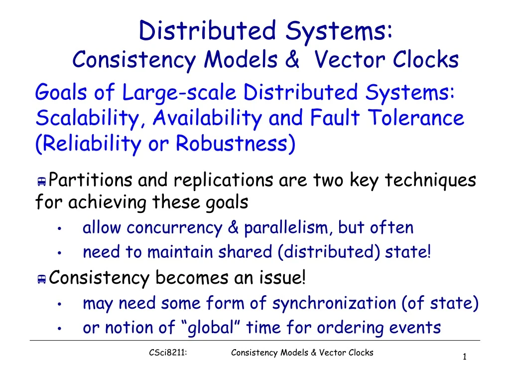
Distributed Systems:Consistency Models & Vector Clocks Goals of Large-scale Distributed Systems: Scalability, Availability and Fault Tolerance (Reliability or Robustness) • Partitions and replications are two key techniques for achieving these goals • allow concurrency & parallelism, but often • need to maintain shared (distributed) state! • Consistency becomes an issue! • may need some form of synchronization (of state) • or notion of “global” time for ordering events CSci8211: Consistency Models & Vector Clocks
Availability, Reliability, Consistency & Performance Trade-offs • Eric Brewer’s CAP Theorem: • In a large-scale distributed system (thus latency & networking issues become critical), we can have all three of the following: consistency, availability and tolerance of network partitions! • Unlike classical single-machine or small cluster systems such as classical relational database systems or networked file systems • Large “real” (operational) large-scale systems sacrifice at least one of these properties: often consistency • e.g., DNS, (nearly all) today’s web services • BASE: Basically Availability, Soft State & Eventual Consistency • What really at stake: latency, failures & performance • large latency makes ensuring strong consistency expensive • availability vs. Consistency: yield (throughput) & harvest (“goodput”)
What is a Consistency Model? • A Consistency Model is a contract between the software and the memory • it states that the memory will work correctly but only if the software obeys certain rules • The issue is how we can state rules that are not too restrictive but allow fast execution in most common cases • These models represent a more general view of sharing data than what we have seen so far! • Conventions we will use: • W(x)a means “a write to x with value a” • R(y)b means “a read from y that returned value b” • “processor” used generically
Strict Consistency • Strict consistency is the strictest model • a read returns the most recently written value (changes are instantaneous) • not well-defined unless the execution of commands is serialized centrally • otherwise the effects of a slow write may have not propagated to the site of the read • this is what uniprocessors support: a = 1; a = 2; print(a); always produces “2” • to exercise our notation: P1: W(x)1 P2: R(x)0 R(x)1 • is this strictly consistent?
Sequential Consistency • Sequential consistency (serializability): the results are the same as if operations from different processors are interleaved, but operations of a single processor appear in the order specified by the program • Example of sequentially consistent execution: P1: W(x)1 P2: R(x)0 R(x)1 • Sequential consistency is inefficient: we want to weaken the model further
Causal Consistency • Causal consistency: writes that are potentially causally related must be seen by all processors in the same order. Concurrent writes may be seen in a different order on different machines • causally related writes: the write comes after a read that returned the value of the other write • Examples (which one is causally consistent, if any?) P1: W(x)1 W(x)3 P2: R(x)1 W(x)2 P3: R(x)1 R(x)3 R(x)2 P4: R(x)1 R(x)2 R(x)3 P1: W(x)1 P2: R(x)1 W(x)2 P3: R(x)2 R(x)1 P4: R(x)1 R(x)2 • Implementation needs to keep dependencies
Pipelined RAM (PRAM) or FIFO Consistency • PRAM consistency is even more relaxed than causal consistency: writes from the same processor are received in order, but writes from distinct processors may be received in different orders by different processors P1: W(x)1 P2: R(x)1 W(x)2 P3: R(x)2 R(x)1 P4: R(x)1 R(x)2 • Slight refinement: • Processor consistency: PRAM consistency plus writes to the same memory location are viewed everywhere in the same order
Weak Consistency • Weak consistency uses synchronization variables to propagate writes to and from a machine at appropriate points: • accesses to synchronization variables are sequentially consistent • no access to a synchronization variable is allowed until all previous writes have completed in all processors • no data access is allowed until all previous accesses to synchronization variables (by the same processor) have been performed • That is: • accessing a synchronization variable “flushes the pipeline” • at a synchronization point, all processors have consistent versions of data
Release Consistency • Release consistency is like weak consistency, but there are two operations “lock” and “unlock” for synchronization • (“acquire/release” are the conventional names) • doing a “lock” means that writes on other processors to protected variables will be known • doing an “unlock” means that writes to protected variables are exported • and will be seen by other machines when they do a “lock” (lazy release consistency) or immediately (eager release consistency)
Eventual Consistency • A form of “weak consistency” – but no explicit notion of synchronization variables • also known as “optimistic replication” • All replicas eventually converge • or making progress toward convergence -- “liveness” guarantee • How to ensure eventual consistency • apply “anti-entropy” measures, e.g., a gossip protocol • apply conflict resolution or “reconciliation”, e.g., last write wins • Conflict resolution often leaves to applications! • E.g., GFS --- not application-transparent, but applications know best! • Strong eventual consistency • Add “saftey” guarantee: i) any two nodes that have received the same (unordered) set of updates will be in the same state; ii) the system is monotonic, the application will never suffer rollbacks. • Using so-called “conflict-free” replicated data types & gossip protocol
Time and Clock • We need to clock to keep “time” so as to order events and to synchronize • Physical Clocks • e.g., UT1, TAI or UTC • physical clocks drift over time -- synch. via, e.g., NTP • can keep closely synchronized, but never perfect • Logical Clocks • Encode causality relationship • Lamport clocks provide only one-way encoding • Vector clocks provide exact causality information
Logical Time or “Happen Before” • Capture just the “happens before” relationship between events • corresponds roughly to causality • Local time at each process is well-defined • Definition (→i): we say e →i e’ if e happens before e’ at process i • Global time (→) --- or rather a global partial ordering: we define e → e’ using the following rules: • Local ordering: e→ e’ if e→ie’ for any process i • Messages: send(m) → receive(m) for any message m • Transitivity: e → e’’ if e→ e’ and e’→ e’’ • We say e“happens before”e’ if e →e’
Currency & Lamport Logical Clocks • Definition of concurrency: • we say e is concurrent with e’ (written e||e’) if neither e→e’ nor e’→e • Lamport clock L orders events consistent with logical “happens before” ordering • if e → e’, then L(e) < L(e’) • But not the converse • L(e) < L(e’) does not imply e → e‘ • Similar rules for concurrency • L(e) = L(e’) implies e║|e’ (for distinct e,e’) • e║|e’ does not imply L(e) = L(e’) • i.e., Lamport clocks arbitrarily order some concurrent events
Lamport’s Algorithm • Each process i keeps a local clock, Li • Three rules: • at process i, increment Li before each event • to send a message m at process i, apply rule 1 and then include the current local time in the message: i.e., send(m,Li) • to receive a message (m,t) at process j, set Lj = max(Lj,t) and then apply rule 1 before time-stamping the receive event • The global time L(e) of an event e is just its local time • for an event e at process i, L(e) = Li(e) • Total-order of Lamport clocks? • many systems require a total-ordering of events, not a partial-ordering • Use Lamport’s algorithm, but break ties using the process ID • L(e) = M * Li(e) + i --- M = maximum number of processes
Vector Clocks • Goal: want ordering that matches causality • V(e) < V(e’) if and only if e → e’ • Method • Label each event by vector V(e) =[c1, c2 …, cn] • ci = # events in process i that causally precede e, n: # of processes • Algorithm: • Initialization: all process starts with V(0)=[0,…,0] • for event on process i, increment own ci • Label message sent with local vector • When process j receives message with vector [d1, d2, …, dn]: • Set local each local entry k to max(ck, dk) • Increment value of cj