ICOM 4036: PROGRAMMING LANGUAGES
Learn about functional programming in Scheme, a dialect of Lisp, and its benefits in software development. Explore the history, syntax, functions, and conditional expressions in Scheme programming.

ICOM 4036: PROGRAMMING LANGUAGES
E N D
Presentation Transcript
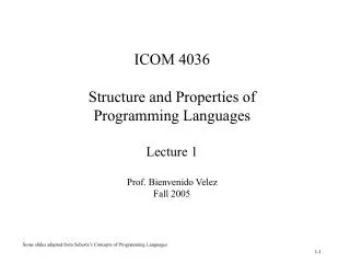
ICOM 4036: PROGRAMMING LANGUAGES Lecture 5 Functional Programming The Case of Scheme 1/6/2020
Required Readings • Texbook (Scott PLP) • Chapter 11 Section 2: Functional Programming • Scheme Language Description • Revised Report on the Algorithmic Language Scheme (available at the course website in Postscript format) At least one exam question will cover these readings
Administrivia • Exam III Date • Tuesday May 10
Functional Programming Impacts Functional programming as a minority discipline in the field of programming languages nears a certain resemblance to socialism in its relation to conventional, capitalist economic doctrine. Their proponents are often brilliant intellectuals perceived to be radical and rather unrealistic by the mainstream, but little-by-little changes are made in conventional languages and economics to incorporate features of the radical proposals. - Morris [1982] “Real programming in functional languages
Functional Programming Highlights • Conventional Imperative Languages Motivated by von Neumann Architecture • Functional programming= New machanism for abstraction • Functional Composition = Interfacing • Solutions as a series of function application f(a), g(f(a)), h(g(f(a))), ........ • Program is an notation or encoding for a value • Computation proceeds by rewriting the program into that value • Sequencing of events not as important • In pure functional languages there is no notion of state
Functional Programming Phylosophy • Symbolic computation / Experimental programming • Easy syntax / Easy to parse / Easy to modify. • Programs as data • High-Order functions • Reusability • No side effects (Pure!) • Dynamic & implicit type systems • Garbage Collection (Implicit Automatic Storage management)
Garbage Collection • At a given point in the execution of a program, a memory location is garbage if no continued execution of the program from this point can access the memory location. • Garbage Collection: Detects unreachable objects during program execution & it is invoked when more memory is needed • Decision made by run-time system, not by the program ( Memory Management).
What’s wrong with this picture? • Theoretically, every imperative program can be written as a functional program. • However, can we use functional programming for practical applications? (Compilers, Graphical Users Interfaces, Network Routers, .....) Eternal Debate: But, most complex software today is written in imperative languages
LISP • Lisp= List Processing • Implemented for processing symbolic information • McCarthy: “Recursive functions of symbolic expressions and their computation by machine” Communications of the ACM, 1960. • 1970’s: Scheme, Portable Standard Lisp • 1984: Common Lisp • 1986: use of Lisp ad internal scripting languages for GNU Emacs and AutoCAD.
History (1) Fortran FLPL (Fortran List Processing Language) No recursion and conditionals within expressions. Lisp (List processor)
History (2) • Lisp (List Processor, McCarthy 1960) * Higher order functions * conditional expressions * data/program duality * scheme (dialect of Lisp, Steele & Sussman 1975) • APL (Inverson 1962) * Array basic data type * Many array operators
History (3) • IFWIM (If You Know What I Mean, Landin 1966) * Infix notation * equational declarative • ML (Meta Language – Gordon, Milner, Appel, McQueen 1970) * static, strong typed language * machine assisted system for formal proofs * data abstraction * Standard ML (1983)
History (4) • FP (Backus 1978) * Lambda calculus * implicit data flow specification • SASL/KRC/Miranda (Turner 1979,1982,1985) * math-like sintax
Scheme: A dialect of LISP • READ-EVAL-PRINT Loop (interpreter) • Prefix Notation • Fully Parenthesized • (* (* (+ 3 5) (- 3 (/ 4 3))) (- (* (+ 4 5) (+ 7 6)) 4)) • (* (* (+ 3 5) (- 3 (/ 4 3))) (- (* (+ 4 5) (+ 7 6)) 4)) A scheme expression results from a pre-order traversal of an expression syntax tree
Scheme Definitions and Expressions • (define pi 3.14159) ; bind a variable to a value pi • pI 3.14159 • (* 5 7 ) 35 • (+ 3 (* 7 4)) 31 ; parenthesized prefix notation
Scheme Functions • (define (square x) (*x x)) square • (square 5) 25 • ((lambda (x) (*x x)) 5) ; unamed function 25 The benefit of lambda notation is that a function value can appear within expressions, either as an operator or as an argument. Scheme programs can construct functions dynamically
Functions that Call other Functions • (define square (x) (* x x)) • (define square (lambda (x) (* x x))) • (define sum-of-squares (lambda (x y) (+ (square x) (square y)))) Named procedures are so powerful because they allow us to hide details and solve theproblem at a higher levelof abstraction.
Scheme Conditional Expressions • (If P E1 E2) ; if P then E1 else E2 • (cond (P1 E1) ; if P1 then E1 ..... (Pk Ek) ; else if Pk then Ek (else Ek+1)) ; else Ek+1 • (define (fact n) (if (equal? n 0) 1 (*n (fact (- n 1))) ) )
Blackboard Exercises • Fibonacci • GCD
Scheme: List Processing (1) • (null? ( )) #t • (define x ‘((It is great) to (see) you)) x • (car x) (It is great) • (cdr x) (to (see) you) • (car (car x)) It • (cdr (car x)) (is great) Quote delays evaluation of expression
Scheme: List Processing (2) • (define a (cons 10 20)) • (define b (cons 3 7)) • (define c (cons a b)) Not a list!! (not null terminated) • (define a (cons 10 (cons 20 ‘())) • (define a (list 10 20) Equivalent
Scheme List Processing (3) • (define (lenght x) (cond ((null? x) 0) (else (+ 1 (length (cdr x)))) )) • (define (append x z) (cond ((null? x) z) (else (cons (car x) (append (cdr x) z ))))) • ( append `(a b c) `(d)) (a b c d)
Backboard Exercises • Map(List,Funtion) • Fold(List,Op,Init) • Fold-map(List,Op,Init,Function)
Scheme: Implemeting Stacks as Lists • Devise a representation for staks and implementations for the functions: push (h, st) returns stack with h on top top (st) returns top element of stack pop(st) returns stack with top element removed • Solution: represent stack by a list push=cons top=car pop=cdr
'(14 (7 () (12()())) (26 (20 (17()()) ()) (31()()))) 14 7 26 12 20 31 17 List Representation for Binary Search Trees
Binary Search Tree Data Type • (define make-tree (lambda (n l r) (list n l r))) • (define empty-tree? (lambda (bst) (null? bst))) • (define label (lambda (bst) (car bst))) • (define left-subtree (lambda (bst) (car (cdr bst)))) • (define right-subtree (lambda (bst) (car (cdr (cdr bst)))))
Searching a Binary Search Tree (define find (lambda (n bst) (cond ((empty-tree? bst) #f) ((= n (label bst)) #t) ((< n (label bst)) (find n (left-subtree bst))) ((> n (label bst)) (find n (right-subtree bst))))))
Recovering a Binary Search Tree Path (define path (lambda (n bst) (if (empty-tree? bst) ‘() ;; didn't find it (if (< n (label bst)) (cons 'L (path n (left-subtree bst))) ;; in the left subtree (if (> n (label bst)) (cons 'R (path n (right-subtree bst))) ;; in the right subtree '() ;; n is here, quit ) ) ) ))
List Representation of Sets { 1, 2, 3, 4 } (list 1 2 3 4) Math Scheme
List Representation of Sets • (define (member? e set) (cond ((null? set) #f) ((equal? e (car set)) #t) (else (member? e (cdr set))) ) ) • (member? 4 (list 1 2 3 4)) > #t
Set Difference (define (setdiff lis1 lis2) (cond ((null? lis1) '()) ((null? lis2) lis1) ((member? (car lis1) lis2) (setdiff (cdr lis1) lis2)) (else (cons (car lis1) (setdiff (cdr lis1) lis2))) ) )
Set Intersection (define (intersection lis1 lis2) (cond ((null? lis1) '()) ((null? lis2) '()) ((member? (car lis1) lis2) (cons (car lis1) (intersection (cdr lis1) lis2))) (else (intersection (cdr lis1) lis2)) ) )
Set Union (define (union lis1 lis2) (cond ((null? lis1) lis2) ((null? lis2) lis1) ((member? (car lis1) lis2) (cons (car lis1) (union (cdr lis1) (setdiff lis2 (cons (car lis1) '()))))) (else (cons (car lis1) (union (cdr lis1) lis2))) ) )
What is Variable? • Imperative view • A variable is an abstraction of a memory (state) cell • Functional view • A variable is an abstraction of a value • Every definition introduces a new variable • Two distinct variables may have the same name • Variables can be characterized as a sextuple of attributes: <name, address, value, type, scope, lifetime>
The Concept of Binding • A Binding is an association, such as between an attribute and an entity, or between an operation and a symbol, or between a variable and a value. • Binding time is the time at which a binding takes place.
Possible Binding Times • Language design time • bind operator symbols to operations • Language implementation time • bind floating point type to a representation • Compile time • bind a variable to a type in C or Java • Load time • bind a FORTRAN 77 variable to a memory cell • a C static variable • Runtime • bind a nonstatic local variable to a memory cell
The Concept of Binding: Static vs. Dynamic • A binding is static if it first occurs before run time and remains unchanged throughout program execution. • A binding is dynamic if it first occurs during execution or can change during execution of the program. We will discuss the choices in selecting binding times for different variable attributes
Design Issues for Names • Maximum length? • Are connector characters allowed? • Are names case sensitive? • Are special words reserved words or keywords? < name, address, value, type, scope, lifetime >
Address or Memory Cell • The physical cell or collection of cells associated with a variable • Also called andl-value • A variable may have different addresses at different times during execution • A variable may have different addresses at different places in a program < name, address, value, type, scope, lifetime >
Aliases • If two variable names can be used to access the same memory location, they are called aliases • Aliases are harmful to readability (program readers must remember all of them) • How can aliases be created: • Pointers, reference variables, C and C++ unions, (and through parameters - discussed in Chapter 9) • Some of the original justifications for aliases are no longer valid; e.g. memory reuse in FORTRAN • Replace them with dynamic allocation
Values • Value – the “object” with which the variable is associated at some point in time • Also known as the r-value of the variable < name, address, value, type, scope, lifetime >
Types • Determines the range of values that a variable may be bound to and the set of operations that are defined for values of that type • Design Issues for Types • When does the binding take place? (Dynamic versus static) • Is the type declared explicitly or implicitly? • Can the programmer create new types? • When are two types compatible? (structural versus name equivalence) • When are programs checked for type correctness? (compile time versus runtime) < name, address, value, type, scope, lifetime >
Scope • The scope of a variable is the range of statements over which it is visible • The nonlocal variables of a program unit are those that are visible but not declared there • The scope rules of a language determine how references to names are associated with variables < name, address, value, type, scope, lifetime >
Static Scope • Binding occurs at compile time • Scope based on program text • To connect a name reference to a variable, you (or the compiler) must find the declaration that is active • Search process: search declarations, first locally, then in increasingly larger enclosing scopes, until one is found for the given name • Enclosing static scopes (to a specific scope) are called its static ancestors; the nearest static ancestor is called a static parent
Static Scope pros and cons • Static scope allows freedom of choice for local variable names • But, global variables can be hidden from a unit by having a "closer" variable with the same name • C++ and Ada allow access to these "hidden" variables • In Ada: unit.name • In C++: class_name::name
Static Scope • Blocks • A method of creating static scopes inside program units--from ALGOL 60 • Examples: C and C++: for (...) { int index; ... } Ada: declare LCL : FLOAT; begin ... end
Static Scope Example • Consider the example: MAIN A B C D E
Static Scope Example Variable X is FREE in A MAIN X:int A … X … C MAIN D A B B X:int E C D E Static links
Static Scope Example Assume: MAIN calls A and B A calls C and D B calls A and E MAIN A B A.K.A Dynamic Function Call Graph C D E Dynamic links