End of Chapter 8
End of Chapter 8. Neil Weisenfeld March 28, 2005. Outline. 8.6 MCMC for Sampling from the Posterior 8.7 Bagging 8.7.1 Examples: Trees with Simulated Data 8.8 Model Averaging and Stacking 8.9 Stochastic Search: Bumping. MCMC for Sampling from the Posterior. Markov chain Monte Carlo method


End of Chapter 8
E N D
Presentation Transcript
End of Chapter 8 Neil Weisenfeld March 28, 2005
Outline • 8.6 MCMC for Sampling from the Posterior • 8.7 Bagging • 8.7.1 Examples: Trees with Simulated Data • 8.8 Model Averaging and Stacking • 8.9 Stochastic Search: Bumping
MCMC for Sampling from the Posterior • Markov chain Monte Carlo method • Estimate parameters given a Bayesian model and sampling from the posterior distribution • Gibbs sampling, a form of MCMC, is like EM only sample from conditional dist rather than maximizing
Gibbs Sampling • Wish to draw a sample from the joint distribution • If this is difficult, but it’s easy to simulate conditional distributions • Gibbs sampler simulates each of these • Process produces a Markov chain with stationary distribution equal to desired joint disttribution
Algorithm 8.3: Gibbs Sampler • Take some initial values • for t=1,2,…: • for k=1,2,…,K generate from: • Continue step 2 until joint distribution of does not change
Gibbs Sampling • Only need to be able to sample from conditional distribution, but if it is known, then: is a better estimate
Gibbs sampling for mixtures • Consider latent data from EM procedure to be another parameter: • See algorithm (next slide), same as EM except sample instead of maximize • Additional steps can be added to include other informative priors
Algorithm 8.4: Gibbs sampling for mixtures • Take some initial values • Repeat for t=1,2,…, • For I=1,2,…,N generate • Set • Continue step 2 until the joint distribution of doesn’t change.
Figure 8.8: Gibbs Sampling from Mixtures Simplified case with fixed variances and mixing proportion
Outline • 8.6 MCMC for Sampling from the Posterior • 8.7 Bagging • 8.7.1 Examples: Trees with Simulated Data • 8.8 Model Averaging and Stacking • 8.9 Stochastic Search: Bumping
8.7 Bagging • Using bootstrap to improve the estimate itself • Bootstrap mean approximately posterior average • Consider regression problem: • Bagging averages estimates over bootstrap samples to produce:
Bagging, cnt’d • Point is to reduce variance of the estimate while leaving bias unchanged • Monte-Carlo estimate of “true” bagging estimate, approaching as • Bagged estimate will differ from the original estimate only when latter is adaptive or non-linear function of the data
Bagging B-Spline Example • Bagging would average the curves in the lower left-hand corner at each x value.
Quick Tree Intro • Can’t do. • Recursive subdivision. • Tree. • f-hat.
Bagging Trees • Each run produces different trees • Each tree may have different terminal nodes • Bagged estimate is the average prediction at x from the B trees. Prediction can be a 0/1 indicator function, in which case bagging gives a pkproportion of trees predicting class k at x.
8.7.1: Example Trees with Simulated Data • Original and 5 bootstrap-grown trees • Two classes, five features, Gaussian distribution • Y from • Bayes error 0.2 • Trees fit to 200 bootstrap samples
Example Performance • High variance among trees because features have pairwise correlation 0.95. • Bagging successfully smooths out vairance and reduces test error.
Where Bagging Doesn’t Help • Classifier is a single axis-oriented split. • Split is chosen along either x1or x2 in order to minimize training error. • Boosting is shown on the right.
Outline • 8.6 MCMC for Sampling from the Posterior • 8.7 Bagging • 8.7.1 Examples: Trees with Simulated Data • 8.8 Model Averaging and Stacking • 8.9 Stochastic Search: Bumping
Model Averaging and Stacking • More general Bayesian model averaging • Given candidate models Mm, m =1…M and a training set Z and • Bayesian prediction is weighted avg of indiv predictions with weights proportional to posterior of each model
Other Averaging Strategies • Simple unweighted average of predictions (each model equally likely) • BIC: use to estimate posterior model probabilities: weight each model depending on fit and how many parameters it uses • Full Bayesian strategy:
Frequentist Viewpoint of Averaging • Given a set of predictions from M models, we seek optimal weights w: • Input x is fixed and N observations in Z are distributed according to P. Solution is the linear regression of Y on the vector of model predictions:
Notes of Frequentist Viewpoint • At the population level, adding models with arbitrary weights can only help. • But the population is, of course, not available • Regression over training set can be used, but this may not be ideal: model complexity not taken into account…
Stacked Generalization, Stacking • Cross validated predictions avoid unfairly high weight to models with high complexity • If w restricted to vectors with one unit weight and the rest zero, model choice has smallest leave-one-out cross validation • In practice we use combined models with optimal weights: better prediction, but less interpretability
Outline • 8.6 MCMC for Sampling from the Posterior • 8.7 Bagging • 8.7.1 Examples: Trees with Simulated Data • 8.8 Model Averaging and Stacking • 8.9 Stochastic Search: Bumping
Stochastic Search: Bumping • Rather than average models, try to find a better single model. • Good for avoiding local minima in the fitting method. • Like bagging, draw bootstrap samples and fit model to each, but choose model that best fits the training data
Stochastic Search: Bumping • Given B bootstrap samples Z*1,…, Z*B, fitting model to each yields predictions: • For squared error, choose model from bootstrap sample: • Bumping tries to move around the model space by perturbing the data.
A contrived case where bumping helps • Greedy tree-based algorithm tries to split on each dimension separately, first one, then the other. • Bumping stumbles upon the right answer.