
Enhancing Lithographic Development Models for Improved Image Quality
Explore the enhanced kinetic development models in optical lithography to optimize dissolution rates and inhibitor concentrations for better resist profiles.

Enhancing Lithographic Development Models for Improved Image Quality
E N D
Presentation Transcript
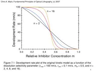
Chris A. Mack, Fundamental Principles of Optical Lithography, (c) 2007 Figure 7.1 Development rate plot of the original kinetic model as a function of the dissolution selectivity parameter (rmax = 100 nm/s, rmin = 0.1 nm/s, mth = 0.5, and n = 2, 4, 8, and 16).
Chris A. Mack, Fundamental Principles of Optical Lithography, (c) 2007 (a) (b) Figure 7.2 Plots of the enhanced kinetic development model for rmax = 100 nm/s, rresin = 10 nm/s, rmin = 0.1 nm/s with: (a) l = 9; and (b) n = 5.
Chris A. Mack, Fundamental Principles of Optical Lithography, (c) 2007 (a) (b) Figure 7.3 An example of a Meyerhofer plot, showing how the addition of increasing concentrations of inhibitor increases rmax and decreases rmin: a) idealized plot showing a log-linear dependence on initial inhibitor concentration, and b) the enhanced kinetic model assuming kenhM0 and kinhM02.
Chris A. Mack, Fundamental Principles of Optical Lithography, (c) 2007 Figure 7.4 Comparison of experimental dissolution rate data (symbols) exhibiting the so-called ‘notch’ shape to best fits of the original (dotted line) and enhanced (solid line) kinetic models. The data shows a steeper drop in development rate at about 0.5 relative inhibitor concentration than either model predicts.
Chris A. Mack, Fundamental Principles of Optical Lithography, (c) 2007 (a) (b) Figure 7.5 Plots of the notch model: (a) mth_notch equal to 0.4, 0.45, and 0.5 with n_notch equal to 30; and (b) n_notch equal to 15, 30, and 60 with mth_notch equal to 0.45.
Chris A. Mack, Fundamental Principles of Optical Lithography, (c) 2007 Figure 7.6 Example surface inhibition with r0 = 0.1 and d = 100 nm for a 1000 nm thick resist.
Chris A. Mack, Fundamental Principles of Optical Lithography, (c) 2007 Figure 7.7 Development rate of THMR-iP3650 (averaged through the middle 20% of the resist thickness) as a function of exposure dose for different developer temperatures shows a change in the shape of the development dose response.
Chris A. Mack, Fundamental Principles of Optical Lithography, (c) 2007 Figure 7.8 Comparison of the best-fit models of THMR-iP3650 for different developer temperatures shows the effect of increasing rmax and increasing dissolution selectivity parameter n on the shape of the development rate curve.
Chris A. Mack, Fundamental Principles of Optical Lithography, (c) 2007 (a) (b) Figure 7.9 Arrhenius plots of the maximum dissolution rate rmax and the dissolution selectivity parameter n for THMR-iP3650.
Chris A. Mack, Fundamental Principles of Optical Lithography, (c) 2007 Figure 7.10 An example Hurter-Driffield (H-D) curve for a photographic negative.
Chris A. Mack, Fundamental Principles of Optical Lithography, (c) 2007 Figure 7.11 Positive resist characteristic curve used to measure contrast.
Chris A. Mack, Fundamental Principles of Optical Lithography, (c) 2007 Figure 7.12 A lithographic H-D curve used to define the theoretical contrast.
Chris A. Mack, Fundamental Principles of Optical Lithography, (c) 2007 Figure 7.13 A typical variation of theoretical contrast with exposure dose. For this data, the FWHM dose ratio is about 5.5.
Chris A. Mack, Fundamental Principles of Optical Lithography, (c) 2007 Figure 7.14 Typical development path.
Chris A. Mack, Fundamental Principles of Optical Lithography, (c) 2007 Figure 7.15 Section of a development path relating path length s to x and z.
Chris A. Mack, Fundamental Principles of Optical Lithography, (c) 2007 Figure 7.16 Example of how the calculation of many development paths leads to the determination of the final resist profile.
Chris A. Mack, Fundamental Principles of Optical Lithography, (c) 2007 (a) (b) Figure 7.17 Matching a three-beam image (a0 = 0.45, a1 = 0.55, a2 = 0.1) with a Gaussian using a) a value of s given by equation (7.91); and b) the best fit s. Note the goodness of the match in the region of the space (x/pitch < 0.25).
Chris A. Mack, Fundamental Principles of Optical Lithography, (c) 2007 (a) (b) Figure 7.18 Simulated aerial images over a range of conditions show that the image log-slope varies about linearly with distance from the nominal resist edge in the region of the space: a) k1 = 0.46 and b) k1 = 0.38 for isolated lines, isolated spaces, and equal lines and spaces and for conventional, annular and quadrupole illumination.
Chris A. Mack, Fundamental Principles of Optical Lithography, (c) 2007 Figure 7.19 A plot of Dawson’s Integral, Dw(z).
Chris A. Mack, Fundamental Principles of Optical Lithography, (c) 2007 Figure 7.20 CD versus dose curves as predicted by the LPM equation (7.98), the LPM using the approximation for the Dawson’s integral, and the VTR. All models assumed a Gaussian image with g = 0.0025 1/nm2 (NILS1 = 2.5 and CD1 = 100 nm), g = 10, and Deff = 200 nm.
Chris A. Mack, Fundamental Principles of Optical Lithography, (c) 2007 (a) (b) Figure 7.21 Measured contrast curves for an i-line resist at development times ranging from 9 to 201 seconds (shown here over two different exposure scales).
Chris A. Mack, Fundamental Principles of Optical Lithography, (c) 2007 Figure 7.22 Analysis of the contrast curves generates an r(m) data set, which was then fit to the original kinetic development model (best fit is shown as the solid line).