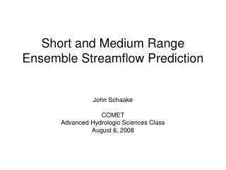
Short and Medium Range Ensemble Streamflow Prediction
Short and Medium Range Ensemble Streamflow Prediction. John Schaake COMET Advanced Hydrologic Sciences Class August 6, 2008. Elements of a Hydrologic Ensemble Prediction System. Ensemble Verification System. QPE, QTE, Soil Moisture. QPF, QTF. Ensemble Pre-Processor.

Short and Medium Range Ensemble Streamflow Prediction
E N D
Presentation Transcript
Short and Medium Range Ensemble Streamflow Prediction John Schaake COMET Advanced Hydrologic Sciences Class August 6, 2008
Elements of a Hydrologic Ensemble Prediction System Ensemble Verification System QPE, QTE, Soil Moisture QPF, QTF Ensemble Pre-Processor Parametric Uncertainty Processor Data Assimilator Hydrology & Water Resources Models Streamflow Ensemble Post-Processor Hydrology & Water Resources Ensemble Product Generator Fig 1
Some Elements of Hydrologic Forecasting ESP forecasts typically are made for many forecast points in a river basin using a distributed (or quasi-distributed) hydrologic model River basins are partitioned into connected segments (which may include elevation zones, reservoirs, river routing segments, etc.) Hydrologic models are calibrated (i.e. parameters are estimated) using historical data Recent observations (precipitation, temperature, SWE, streamflow are used to estimate inititial conditions at the time a forecast is created.
ESP Forecast Process Raw Atmospheric Forecasts EPP Intitial Conditions ESP Raw ESP Hydrographs Model Parameters
ESP Input Requirements • Forecast precipitation and temperature ensemble forcing: • For every forecast segment • Member time series at ~6hr step for entire forecast period • Individual members must be “consistent” over all segments and for the entire forecast period.
ESP Input Requirements (cont’d) • Statistical Properties: • Ensembles must be unbiased at all time and space scales and for all lead times • Ensembles must account for space/time scale dependency in the variability of precipitation and temperature and in the forecast uncertainty at all space and time scales • Each member must be equally likely to occur (i.e. a random sample)
precip. depth (mm) precip. depth (mm) 4a 4b space (HRAP bins) space (HRAP bins) precip. depth (mm) precip. depth (mm) 4d space (HRAP bins) 4c space (HRAP bins)
Hydrology is Sensitive to Precipitation Variability:Spatial Scale Dependency Example • Total runoff from 64x64 4km grid domain • Several years of Stage III, 1-hr, QPE • 7 Area Segmentations: 1,2,4,6,16,32,64 pixels • Same model/parameters used for each segmentation • Graph shows different runoff totals vs size of area segment • Some models more scale dependent than others • Scale dependency is a result of non-linearity THEREFORE: Space/Time Variability of Ensemble Forcing Will Have a Primary Effect on Hydrologic Ensemble Response
Example EnsembleInputs and ESP OutputforAmerican River Basin, CA
Raw Atmospheric ForecastsViewed from aHydrologic Perspective
Uncertainty Analysis of Global Ensemble Precipitation Forecasts
Illustration of the scale-dependent skill in GFS ensemble mean winter season precipitation forecasts for the North Fork of the American River Basin.The curve labeled “moving 6hr window” shows how the correlation between 6hr precipitation forecasts and corresponding observations decreases with increasing forecast lead time.The curve labeled “average from t=0” shows the correlations averages accumulated over windows beginning at t=0 and corresponding observations decreases as the time to the end of the window increases. The remaining curves are for similar averages that begin at different times after t=0. Fig 5
Forecast Window Width (6-hr periods) Forecast Lead Time to Beginning of Forecast Window (6-hr periods) GFS Precipitation Forecast Correlation Coefficient: Temporal Scale-DependencyNFDC1HUP – January 15 Forecasts 2 weeks Increasing lead time to end of forecast period 1 week
Ensemble Pre-Processor (EPP)Objectives • Produce ensemble forcing for ESP • Remove bias in atmospheric forecasts • Correct spread problems • Preserve space-time variability and uncertainty structure • Downscale atmospheric to forecast basins
EPP2 – Step Process Raw Atmospheric Forecasts Estimate Probability Distributions This step includes downscaling, and correction of bias and spread problems This step assures that members are “consistent” over all basins for the entire forecast period Assign Values to Ensemble Members ESP Input Forcing (Schaake Shuffle)
Estimate Probability Distributionsfor each: Time-step, Aggregate Sub-period and Forecast Sub-Area (segment) • Use historical single-value forecasts and observations (for a common period of time)
Estimate Probability Distributions(Cont’d) • Estimate climatological distributions of forecasts and observations • Use climatologies to transform forecasts and observations to Standard Normal Deviates • Estimate correlation parameter of Joint Distribution
Calibration PDF of STD Normal PDF of Observed Joint distribution Sample Space Y NQT Observed Correlation(X,Y) Joint distribution X Y 0 Model Space Forecast PDF of Forecast PDF of STD Normal Observed NQT X Forecast National DOH Workshop, Silver Spring, MD July 15-17, 2008
Ensemble Generation Conditional distribution given xfcst Joint distribution Model Space Y 1 Observed x1 Ensemble members … Probability xn xfcst X Forecast 0 x1 xi xn Ensemble forecast Obtain conditional distribution given a single-value forecast xfcst National DOH Workshop, Silver Spring, MD July 15-17, 2008
Use EPP Forecast Probability Distributions to Assign Values to Members) • Divide total forecast period into sub-periods for: • Individual time-steps • Aggregate time periods • Estimate forecast probability distribution for each time-step and each sub-period • Construct ensemble members using “Schaake Shuffle” • Resolve differences between member values for aggregate periods and time-step periods Example Cascade Of Sub-Periods Aggregate periods Individual time steps
Schaake Shuffle For each segment, at each time step, associate forecast ensemble members (left panel) with historical ensemble members (right panel) by rank (and hence year) Conditional distribution given xfcst Historical ensemble distribution 1 1 Probability Probability 0 0 y1 yi yn x1 xi xn (1996) (1996) Historical Ensemble Forecast Ensemble National DOH Workshop, Silver Spring, MD July 15-17, 2008
Operational RFC QPF Files Operational RFC QTF Files Operational GFS Files Operational GFS Files Operational Forecast Files Operational Forecast Files MAT Time Series Identifiers MAT Area Locations Stations used for MAT Analysis Temperature Normals MAP Area Locations MAP Time Series Identifiers National Weather Service Hydrologic Ensemble Pre-Processor (EPP) GFS Subsystem J. Schaake, R. Hartman, J. Demargne, L. Wu, M. Mullusky, E. Welles, H. Herr, D. J. Seo, and P. Restrepo Average observed values of 6-hour precipitation corresponding to RFC and GFS forecasts Continuous Rank Probability Skill Score (CRPSS) for 6-hour precipitation forecasts Pre-ProcessorPrecipitation Algorithms Historical 6hr RFC Operational MAP Observed Data Files RFC single-value forecasts (mm) 6hr RFC QPF Verifications Files and Operational MAPs RFC-specific Utility Historical 6hr RFC Operational MAP QPF Data files Operational Ensemble MAPs Historical GFS Ensemble Mean Precipitation Forecasts (mm) Ensemble forecasts based on RFC single-value forecasts Precipitation Parameters Ensemble Generator Parameter Estimator 6hr MAP Calibration Files 6hr MAP Unformatted Calibration Data Files Hindcast Ensemble MAPs MAP Conversion Utility Raw Historical Data Files GFS Processor Historical Data Sets Average forecast values of 6-hour precipitation for RFC and GFS GFS single-value forecasts (mm) Precipitation Verification Index Files Data Analysis Ensemble forecasts based on GFS single-value forecasts CFS Ensemble Forecast (Application Under Construction) (mm) Verification Results Statistics Precipitation Ensemble Pre-Processor Average observed values of daily minimum temperature corresponding to RFC and GFS forecasts Continuous Rank Probability Skill Score (CRPSS) for daily minimum temperature forecasts RFC Historical Operational Observed TMX/TMN Pre-Processor Temperature Algorithms RFC single-value forecasts RFC TMX/TMN Forecast Verification Files and Operational Observed TMX/TMN RFC-specific Utility RFC Historical Operational Forecast TMX/TMN MAT Analysis Operational Ensemble MATs MOS TMX/TMN Forecast Verification Files MOS Historical Forecast TMX/TMN MOS Utility Ensemble forecasts based on RFC single-value forecasts Temperature Parameters Parameter Estimator Ensemble Generator Hindcast Ensemble MATs Average forecast values of daily minimum temperature for RFC and GFS 6hr MAT Calibration Files 6hr to TMX/TMN GFS single-value forecasts Historical GFS Ensemble Mean Temperature Forecasts Raw Historical Data Files Temperature Verification TMX/TMN Calibration Data Index Files Ensemble forecasts based on GFS single-value forecasts Unformatted TMX/TMN Calibration Data Files Conversion Utility Verification Results GFS Processor Historical Data Sets CFS Ensemble Forecast (Application Under Construction) Temperature Ensemble Pre-Processor TMX: maximum temperature TMN: minimum temperature
CNRFC Ensemble Prototype Smith River Mad River Salmon River Van Duzen River American River (11 basins) Navarro River
Some EPP ParametersNorth Fork American River Observed POP Observed CAVG Forecast CAVG Forecast POP
Correlation CoefficientGFS Precipitation Forecast vs ObservationNorth Fork American River Forecast Uncertainty Depends on both Lead-Time and Aggregation- Time Aggregate periods
Bias – NFDC1HUF Precipitation Raw Forecasts Ensemble Mean RFC Forecasts GFS Forecasts
GFS Precipitation Forecast Verification North Fork American River Raw GFS Ensemble Mean GFS EPP Prototype Bias Day of Year Day of Year CRPSS Forecast Period Forecast Period
Short-term Ensemble PrototypeNF American (upper subarea)5-day Temperature Ensembles
Short-term Ensemble PrototypeNF American (upper subarea)5-day Precipitation Ensembles QPF = 1.5 inches in two successive 6-hr periods, otherwise zero
Short-term Ensemble PrototypeNF American 5-day Streamflow Ensembles
Short-term Ensemble PrototypeNF American5-day Streamflow Distribution