Schemata Theory
250 likes | 294 Vues
Explore the application of schema theory in genetic algorithm optimization, understanding similarity, and fitness estimation.

Schemata Theory
E N D
Presentation Transcript
Schemata Theory Chapter 11
Why Bother with Theory? • Might provide performance guarantees • Convergence to the global optimum can be guaranteed providing certain conditions hold • Might aid better algorithm design • Increased understanding can be gained about operator interplay etc. • Mathematical Models of EAs also inform theoretical biologists • Because you never know ….
What Approach? • Define similarity among individuals • Study evolution of similarities between candidate solutions • Study evolution of groups of similar candidate solutions
How Can We Describe Similarity? • To describe similarity among individuals in the population we use the concept of schema (schemata) • What is a schema? • Similarity template describing a subset of strings • String over the alphabet {0,1,*} • * is the don’t care symbol • The don’t care symbol * is a metasymbol: • it is never explicitly process by the genetic algorithm
Basic Idea The idea of a schema: how can we represent a subset of the population whose individuals all share some characteristics? In case the chromosomes are represented by fixed-length strings over a finite alphabet, a schema is a pattern, of the same length as a chromosome, some of whose positions are filled by elements of the alphabet and some by “don’t care” symbols. If the alphabet is a binary alphabet, a schema could be represented as (* * * 1 * * 0 0 * * 1) indicating any string of 11 binary digits with ones and zeros in the positions indicated, and anything at all (zeros or ones) in the positions containing an asterisk.
Holland’s Schema Theorem (1975) • A schema (pl. schemata) is a string in a ternary alphabet ( 0,1 # = “don’t care”) representing a hyperplane within the solution space. • E.g. 0001# #1# #0#, ##1##0## etc • Two values can be used to describe schemata, • the Order (number of defined positions) = 6,2 • the Defining Length - length of sub-string between outmost defined positions = 9, 3
Examples of Schema • Schema ***11 matches, • 00011 • 00111 • 01011 • … • 11111 • Schema 0***1 matches, • 00001 • 00011 • 00101 • … • 01111
Schema and Schemata (I) • • Order of schema H, o(H) • the number of specific (non-*) positions in the schema • Examples • - o(**1*0) = 2 • - o(1**11) = 3 • Defining length of schema H, δ(H) • distance between first and last non-* in a schema • Examples • - δ(**1*0) = 2 • - δ(1**11) = 4
Schema and Schemata (II) • • Schema H1 is a competitor of schema H2 if, • H1 and H2 are specified in the same positions. • H1 and H2 differ in at least one specified position. • • Example • *111* is a competitor of *101* • Any string of length l is an instance of 2^l (2l) different schemas. • Implicit parallelism • One string’s fitness tells us something about the relative • fitness of more than one schema.
111 01# 1## 001 100 10# 000 xzy Example Schemata H o(H) d(H) 001 3 2 01# 2 1 1#0 2 2 1## 1 0
How a Simple Genetic Algorithm Works? • A simple genetic algorithm • Population size N • Fixed-length binary strings of length l • Fitness-proportionate selection • One-point crossover with probability pc • Bit-flip mutation • Fitness is positive • How selection, crossover, and mutation work?
Notations used • Let H be a schema with at least one instance in the population at time t. • Let m(H, t) be the number of instances of H at time t. • Let f(H, t) be the observed (based on the sample) average fitness of (the strings of) H at time t. • Let f(x) be the fitness of a string x; let <f(t)> be the average fitness of the population at time t. • We want to calculate E(m(H, t + 1)), the expected number of instances of H at time t + 1.
Schema Fitnesses (I) • The true “fitness” of a schema H is taken by averaging over all possible values in the “don’t care” positions, but this is effectively sampled by the population, giving an estimated fitness f(H, t).
Schema Fitnesses (I) - Exercise • While optimizing a 4-bit problem, you notice that your population, of size 400, consists of 123 copies of genome 0001 (with fitness 0.12), 57 copies of genome 1111 (with fitness 0.23), 201 copies of genome 1010 (with fitness 0.56), and 19 copies of genome 0110 (with fitness 0.43). • What is the estimated fitness of schema H=1***? Answer: The estimated fitness of schema 1*** is: f(H, t) = ( 57*0.23+201*0.56)/(57+201) = 0.4870
Schema Fitnesses (II) • With Fitness Proportionate Selection, the expected number of offspring of a string x at time t is equal to f(x) / <f(t)> proportion of H in next parent pool is: E(m(H,t+1)) = m(H,t) * f(H,t) / <f(t)> E or , in other words: where x ÎH denotes “x is an instance of H”.
Schema Fitnesses (II) - continued • Assuming that H is a scheme that at the t generation has a fitness greater than <f(t)> (the population average fitness) iff(H,t)/<f(t)> >1 thenE(m(H,t+1)) > m(H,t) • A schema that has performance above average will have more representatives in the next generation population. • With Fitness Proportionate Selection, the number of representatives for a schema that hasfitness rate above average, increases exponentially.
Schema Fitnesses (II) - Exercise • While optimizing a 4-bit problem, you notice that your population, of size 400, consists of 123 copies of genome 0001 (with fitness 0.12), 57 copies of genome 1111 (with fitness 0.23), 201 copies of genome 1010 (with fitness 0.56), and 19 copies of genome 0110 (with fitness 0.43). • Assuming fitness-proportionate selection with no crossover or mutation, calculate the estimated fitness of this schema (1***) in the next generation. Answer: Let S1 = 1111, S2 = 1010 and <f(t)> – the average fitness of population in time t <f(t)>=( 57*0.23+201*0.56+123*0.12+19*0.43)/400 = 0.3715 E(m(S1,t+1)) = m(S1,t) * f(S1,t) / <f(t)> = 57*0.23 / 0.3715 = 35.289 E(m(S2,t+1)) = m(S2,t) * f(S2,t) / <f(t)> = 201*0.56 / 0.3715 = 302.987 E(m(H,t+1)) = m(H,t) * f(H,t) / <f(t)> E =258*0.4870 / 0.3715 = 338.21 Hence, the estimated fitness of schema H=1*** is: f(H, t) = (35.289 *0.23+ 302.987 *0.56)/(35.289 + 302.987) = 0.5255
Schema Disruption I • One Point Crossover selects a crossover point at random from the l-1 possible points (where l is the length of the schema – number of bits to represent each chromosome) • For a schema with defining length d the random point will fall inside the schema with probability = d(H) / (l-1). • If recombination is applied with probability Pc the survival probability is 1.0 - Pc*d(H)/(l-1)
Schema Disruption II • The probability that bit-wise mutation with probability Pm will NOT disrupt the schemata is simply the probability that mutation does NOT occur in any of the defining positions, Psurvive (mutation) = ( 1- Pm)o(H) = 1 – o(H) * Pm + terms in Pm2 +… where o(H)is the Order of H schema (number of defined positions) • For low mutation rates, this survival probability under mutation approximates to 1 - o(H)*Pm
Schema Survival • The probability that the schema survives both crossover and mutation is: Psurvive (crossover) * Psurvive (mutation) = = [1 - Pc*d(H)/(l-1)] * ( 1- Pm)o(H)
The Schema Theorem (I) • Put together, the proportion of a schema H in successive generations varies as: • Condition for schema to increase its representation is: • Inequality is due to convergence affecting crossover disruption, exact versions have been developed
The Schema Theorem (II) • Two factors influence the number of representatives of H • Over the average schema fitness, leads to higher m(H,t+1) • Greater o(H) and δ(H), lead to a smaller m(H,t+1) • Highly fit, short, low order schemata become the partial solutions to a problem (these are called building-blocks) • By processing similarities, a genetic algorithm reduces the complexity of an arbitrary problems
Criticisms of the Schema Theorem • It presents an inequality that does not take into account the constructive effects of crossover and mutation • Exact versions have been derived • Have links to Price’s theorem in biology • Because the mean population fitness, and the estimated fitness of a schema will vary from generation to generation, it says nothing about gen. t+2 etc. • “Royal Road” problems constructed to be GA-easy based on schema theorem turned out to be better solved by random mutation Hill-Climbers • BUT it remains a useful conceptual tool and has historical importance
Building Blocks • Low order, low defining-length schemata with above average fitness. Building Block Hypothesis • “Short, low-order, and highly fit schemata are sampled, recombined, and resampled to form strings of potentially higher fitness […] we construct better and better strings from the best partial solutions of the past samplings.” David Goldberg, 1989
How Many Schemata are Processed? • A population with size n (individuals) and the individual’s length l processes between 2^l (2l) to nx 2l schemata. • Consider only schemata that survive with a certain probability. • Count how many schemata are effectively processed • Effective processing = selection + mixing (recombination). • Implicit Parallelism (J. Holland) • A genetic algorithm with a population size n can usefully process on the order of O(n3) schemata in a generation despite the processing of only n solutions
