Download
1 / 19
190 likes | 312 Vues
Forward and Inverse Modeling of Ocean Color. Tihomir Kostadinov Maeva Doron Radiative Transfer Theory SMS 598(4) Darling Marine Center, University of Maine, USA July 2004. Acknowledgements. Maeva Doron for working together, and giving me one more reason to visit Southern France.

E N D
Forward and Inverse Modeling of Ocean Color Tihomir Kostadinov Maeva Doron Radiative Transfer Theory SMS 598(4) Darling Marine Center, University of Maine, USA July 2004
Acknowledgements • Maeva Doron for working together, and giving me one more reason to visit Southern France. • The funding agencies – ONR, NASA, UM, etc. • Curtis Mobley for the project idea and assistance, and for the fabulous lectures, the dedication, and for the mathematics. • Emmanuel Boss and Collin Roesler for similar reasons (also MJ Perry for SMS 598(3)) • Trisha and others “behind the scenes” who made this possible • ME weather, which fulfilled my dreams of lots of • The meadows and the forests, for being soooo reflective in the 550 nm range. And so serene and beautiful • The Damariscotta river and the Atlantic for smelling so nice, and heading such an impressive tidal range. • The HTSRB and the HyperPro buoys for being cute and hyperspectral. RAIN
Outline • Part I SSA approximation (forward) • Part II the GSM algorithm, sensitivity analysis for two reflectances.
Introduction • Complicated to solve in 3D in its full differential glory • We need practical approximations for FORWARD modeling to link water constituents IOPs AOPs Remotely sensed ocean color. • Having a functional relationship (not necessarily analytical) will let us use the INVERSE model to estimate biogeochemical parameters from Rrs
L’équation du transfert radiatif • Single Scattering Approximation (SSA) • Ignore all terms in infinite series after the first scattering term • Quasi-SSA if forward scattering is counted as unscattered light famousRrs = f(bb/(a+bb)) relationship
The SSA • Hydrolight runs for wo = 0.001, 0.01,0.1,0.3,0.5,0.7,0,9 • Idealized black sky with sun zenith angle 42.1 (30 in the water), calm seas (no wind), at = 0.8 1/m homogeneous; infinite bottom. • Coded the SSA solution (as given by Mobley lecture) for the same inputs and the same quad discretization as HL. • Compare SSA performance against HL for the different wo.
The Garver Siegel Maritorena model • Semianalytical, l = [412,443,490,510,555] • Retrievals are 3: [chl], ag(443) + ad(443), bbp(443) • Parameters are 7: specific Chl a, slope of CDOM (S), slope of backscattering (η). • Tuned by simulated annealing for the global ocean (Maritorena et al. 2002) • Sensitivity analysis for S and η follows. aphi* left as tuned in Maritorena et al. 2002
Station B – off of Pemaquid Pt. 23-Jul-04 lat:43:48.06 lon:69:32.63 time:15:55