
Quicksort
E N D
Presentation Transcript
Quicksort Ack: Several slides from Prof. Jim Anderson’s COMP 750 notes.
Performance • A triumph of analysis by C.A.R. Hoare • Worst-case execution time – (n2). • Average-case execution time – (n lg n). • How do the above compare with the complexities of other sorting algorithms? • Empirical and analytical studies show that quicksort can be expected to be twice as fast as its competitors.
Design • Follows the divide-and-conquer paradigm. • Divide:Partition (separate) the array A[p..r] into two (possibly empty) subarrays A[p..q–1] and A[q+1..r]. • Each element in A[p..q–1] A[q]. • A[q] each element in A[q+1..r]. • Index q is computed as part of the partitioning procedure. • Conquer: Sort the two subarrays by recursive calls to quicksort. • Combine: The subarrays are sorted in place – no work is needed to combine them. • How do the divide and combine steps of quicksort compare with those of merge sort?
Pseudocode Partition(A, p, r) x, i := A[r], p – 1; for j := p to r – 1 do if A[j] x then i := i + 1; A[i] A[j] fi od; A[i + 1] A[r]; return i + 1 Quicksort(A, p, r) if p < r then q := Partition(A, p, r); Quicksort(A, p, q – 1); Quicksort(A, q + 1, r) fi A[p..r] 5 A[p..q – 1] A[q+1..r] Partition 5 5 5
Partitioning • Select the last element A[r] in the subarray A[p..r] as the pivot– the element around which to partition. • As the procedure executes, the array is partitioned into four (possibly empty) regions. • A[p..i] — All entries in this region are pivot. • A[i+1..j – 1] — All entries in this region are > pivot. • A[r] = pivot. • A[j..r – 1] — Not known how they compare to pivot. • The above hold before each iteration of the for loop, and constitute a loop invariant. (4 is not part of the LI.)
Example p r initially: 2 5 8 3 9 4 1 7 10 6note: pivot (x) = 6 i j next iteration:2 5 8 3 9 4 1 7 10 6 i j next iteration:25 8 3 9 4 1 7 10 6 i j next iteration:2 58 3 9 4 1 7 10 6 i j next iteration:2 538 9 4 1 7 10 6 i j Partition(A, p, r) x, i := A[r], p – 1; for j := p to r – 1 do if A[j] x then i := i + 1; A[i] A[j] fi od; A[i + 1] A[r]; return i + 1
Example (Continued) next iteration:2 538 9 4 1 7 10 6 i j next iteration:2 5389 4 1 7 10 6 i j next iteration:2 534 98 1 7 10 6 i j next iteration:2 534189 7 10 6 i j next iteration:2 5341897 10 6 i j next iteration:2 5341897106 i j after final swap:2 5341697108 i j Partition(A, p, r) x, i := A[r], p – 1; for j := p to r – 1 do if A[j] x then i := i + 1; A[i] A[j] fi od; A[i + 1] A[r]; return i + 1
Partitioning • Select the last element A[r] in the subarray A[p..r] as the pivot– the element around which to partition. • As the procedure executes, the array is partitioned into four (possibly empty) regions. • A[p..i] — All entries in this region are pivot. • A[i+1..j – 1] — All entries in this region are > pivot. • A[r] = pivot. • A[j..r – 1] — Not known how they compare to pivot. • The above hold before each iteration of the for loop, and constitute a loop invariant. (4 is not part of the LI.)
Correctness of Partition • Use loop invariant. • Initialization: • Before first iteration • A[p..i] and A[i+1..j – 1] are empty – Conds. 1 and 2 are satisfied (trivially). • r is the index of the pivot – Cond. 3 is satisfied. • Maintenance: • Case 1:A[j] > x • Increment j only. • LI is maintained. Partition(A, p, r) x, i := A[r], p – 1; for j := p to r – 1 do if A[j] x then i := i + 1; A[i] A[j] fi od; A[i + 1] A[r]; return i + 1
i r j p >x x > x x j i r p x > x x Correctness of Partition Case 1: A[j] > x
i r j p x x > x x i j r p x > x x Correctness of Partition • A[r] is unaltered. • Condition 3 is maintained. • Case 2:A[j] x • Increment i • Swap A[i] and A[j] • Condition 1 is maintained. • Increment j • Condition 2 is maintained.
Correctness of Partition • Termination: • When the loop terminates, j = r, so all elements in A are partitioned into one of the three cases: • A[p..i] pivot • A[i+1..j – 1] > pivot • A[r] = pivot • The last two lines swap A[i+1] and A[r]. • Pivot moves from the end of the array to between the two subarrays. • Thus, procedure partition correctly performs the divide step.
Complexity of Partition • PartitionTime(n) is given by the number of iterations in the for loop. • (n) : n = r – p + 1. Partition(A, p, r) x, i := A[r], p – 1; for j := p to r – 1 do if A[j] x then i := i + 1; A[i] A[j] fi od; A[i + 1] A[r]; return i + 1
Algorithm Performance Running time of quicksort depends on whether the partitioning is balanced or not. • Worst-Case Partitioning (Unbalanced Partitions): • Occurs when every call to partition results in the most unbalanced partition. • Partition is most unbalanced when • Subproblem 1 is of size n – 1, and subproblem 2 is of size 0 or vice versa. • pivot every element in A[p..r – 1] or pivot< every element in A[p..r – 1]. • Every call to partition is most unbalanced when • Array A[1..n] is sorted or reverse sorted!
Worst-case Partition Analysis Recursion tree for worst-case partition n Running time for worst-case partitions at each recursive level: T(n) = T(n – 1) + T(0) + PartitionTime(n) = T(n – 1) + c·n = 1≤k≤ n c·k = c( 1≤k≤ nk ) = (n2) n – 1 n – 2 n n – 3 2 1
Best-case Partitioning • Size of each subproblem n/2. • One of the subproblems is of size n/2 • The other is of size n/2 1. • Recurrence for running time • T(n) 2T(n/2) + PartitionTime(n) = 2T(n/2) + c·n • T(n) = (n lg n)
cn cn/2 cn/2 cn/4 cn/4 cn/4 cn/4 c c c c c c Recursion Tree for Best-case Partition cn cn lg n cn cn Total : O(n lg n)
Randomized Quicksort • Want to make running time independent of input ordering. • How can we do that? • Make the algorithm randomized. • Make every possible input equally likely. • Can randomly shuffle to permute the entire array. • For quicksort, it is sufficient if we can ensure that every element is equally likely to be the pivot. • So, we choose an element in A[p..r] and exchange it with A[r]. • Because the pivot is randomly chosen, we expect the partitioning to be well balanced on average.
Variations (Continued) • Input distribution may not be uniformly random. • Fix 1:Use “randomly” selected pivot. • We’ll analyze this in detail. • Fix 2:Median-of-three Quicksort. • Use median of three fixed elements (say, the first, middle, and last) as the pivot. • To get O(n2) behavior, we must continually be unlucky to see that two out of the three elements examined are among the largest or smallest of their sets.
Randomized Version Want to make running time independent of input ordering. Randomized-Partition(A, p, r) i := Random(p, r); A[r] A[i]; Partition(A, p, r) Randomized-Quicksort(A, p, r) if p < r then q := Randomized-Partition(A, p, r); Randomized-Quicksort(A, p, q – 1); Randomized-Quicksort(A, q + 1, r) fi Partition(A, p, r) x, i := A[r], p – 1; for j := p to r – 1 do if A[j] x then i := i + 1; A[i] A[j] fi od; A[i + 1] A[r]; return i + 1