Maximizing Performance with IBM DataStar Tools Overview
Explore a comprehensive overview of IBM DataStar tools for parallel processing, performance monitoring, and access optimization. Learn about batch and interactive computing, job queues, system access modes, and hardware performance monitoring. Dive into the details of IBM Power systems with parallel processing nodes, memory configurations, and specialized tools like HPM and PMAPI. Discover the significance of hardware counters, performance monitors, and metrics such as MIPS and MFLOPS. Gain insights into hardware performance measurement techniques and tools like HPM Toolkit for optimizing application performance efficiently. Enhance your understanding of performance monitoring, system activity measurement, and hardware counter motivations. With a focus on maximizing efficiency and utilization, leverage the power of IBM DataStar tools for high-performance computing needs.

Maximizing Performance with IBM DataStar Tools Overview
E N D
Presentation Transcript
Using parallel tools on the SDSC IBM DataStar • DataStar Overview • HPM • Perf • IPM • VAMPIR • TotalView
DataStar Overview • P655 :: ( 8-way, 16GB) 176 nodes • P655+ :: ( 8-way, 32GB) 96 nodes • P690 :: ( 32-way, 64GB) 2 nodes • P690 :: ( 32-way, 128GB) 4 nodes • P690 :: ( 32-way, 256GB) 2 nodes Total – 280 nodes :::: 2,432 processors.
Batch/Interactive computing • Batch Job Queues: • Job queue Manager – Load Leveler (tool from IBM) • Job queue Scheduler – Catalina (SDSC internal tool) • Job queue Monitoring – Various tools (commands) • Jobs Accounting – Job filter (SDSC internal PERL scripts)
DataStar Access • Three Login Nodes :: Access modes (platforms) (usage mode) • dslogin.sdsc.edu :: Production runs (P690, 32-way, 64GB) • dspoe.sdsc.edu :: Test/debug runs (P655, 8-way, 16GB) • dsdirect.sdsc.edu :: Special needs (P690, 32-way, 256GB) Note : Above Usage modes division is not very strict.
Test/debug runs (Usage from dspoe) [dspoe.sdsc.edu :: P655, 8-way, 16GB] • Access to two queues: • P655 nodes [shared] • P655 nodes [Not – shared] • Job queues have Job filter + Load Leveler only (very fast) • Special command line submission (along with job script).
Production runs (Usage from dslogin) [dslogin.sdsc.edu :: P690, 32-way, 64GB] • Data transfer/ Src editing/Compliation etc… • Two queues: • Onto p655/p655+ nodes [not shared] • Onto p690 nodes [shared] • Job ques have Job filter + LoadLeveler + Catalina (Slowupdates)
All Special needs (Usage from dsdirect) [dsdirect.sdsc.edu :: P690, 32-way, 256GB] • All Visualization needs • All post data analysis needs • Shared node (with 256 GB of memory) • Process accounting in place • Total (a.out) interactive usage. • No Job filter, No Load Leveler, No Catalina
What is Performance? - Where is time spent and how is time spent? • MIPS – Millions of Instructions Per Second • MFLOPS – Millions of Floating-Point Operations Per Second • Run time/CPU time
What is a Performance Monitor? • Provides detailed processor/system data • Processor Monitors • Typically a group of registers • Special purpose registers keep track of programmable events • Non-intrusive counts result in “accurate” measurement of processor events • Typical Events counted are Instruction, floating point instruction, cache misses, etc. • System Level Monitors • Can be hardware or software • Intended to measure system activity • Examples: • bus monitor: measures memory traffic, can analyze cache coherency issues in multiprocessor system • Network monitor: measures network traffic, can analyze web traffic internally and externally
Hardware Counter Motivations • To understand execution behavior of application code • Why not use software? • Strength: simple, GUI interface • Weakness: large overhead, intrusive, higher level, abstraction and simplicity • How about using a simulator? • Strength: control, low-level, accurate • Weakness: limit on size of code, difficult to implement, time-consuming to run • When should we directly use hardware counters? • Software and simulators not available or not enough • Strength: non-intrusive, instruction level analysis, moderate control, very accurate, low overhead • Weakness: not typically reusable, OS kernel support
Ptools Project • PMAPI Project • Common standard API for industry • Supported by IBM, SUN, SGI, COMPAQ etc • PAPI Project • Standard application programming interface • Portable, available through a module • Can access hardware counter info • HPM Toolkit • Easy to use • Doesn’t effect code performance • Use hardware counters • Designed specifically for IBM SPs and Power
Problem Set • Should we collect all events all the time? • Not necessary and wasteful • What counts should be used? • Gather only what you need • Cycles • Committed Instructions • Loads • Stores • L1/L2 misses • L1/L2 stores • Committed fl pt instr • Branches • Branch misses • TLB misses • Cache misses
IBM HPM Toolkit • High Performance Monitor • Developed for performance measurement of applications running on IBM Power3 systems. It consists of: • An utility (hpmcount) • An instrumentation library (libhpm) • A graphical user interface (hpmviz). • Requires PMAPI kernel extensions to be loaded • Works on IBM 630 and 604e processors • Based on IBM’s PMAPI – low level interface
HPM Count • Utilities for performance measurement of application • Extra logic inserted to the processor to count specific events • Updated at every cycle • Provide a summary output at the end of the execution: • Wall clock time • Resource usage statistics • Hardware performance counters information • Derived hardware metrics • Serial/Parallel, Gives each performance numbers for each task
Timers Time usually reports three metrics: • User Time • The time used by your code on CPU, also CPU time • Total time in user mode = Cycles/Processor Frequency • System Time • The time used by your code running kernel code (doing I/O, writing to disk, or printing to the screen etc). • It is worth to minimize the system time, by speeding up the disk I/O, doing I/O in parallel, or doing I/O in background while your CPU computes in the foreground • Wall Clock time • Total execution time, the combination of the time 1 and 2 plus the time spent idle (waiting for resources) • In parallel performance tuning, only wall clock time counts • Interprocessor communication consumes a significant amount of your execution time (user/system time usually don’t account for it), need to rely on wall clock time for all the time consumed by the job
Floating Point Measures • PM_FPU0_CMPL (FPU 0 instructions) • The POWER3 processor has two Floating Point Units (FPU) which operate in parallel. Each FPU can start a new instruction at every cycle. This counter shows the number of floating point instructions that have been executed by the first FPU. • PM_FPU1_CMPL (FPU 1 instructions) • This counter shows the number of floating point instructions (add, multiply, subtract, divide, multiply & add) that have been processed by the second FPU. • PM_EXEC_FMA (FMAs executed) • This is the number of Floating point Multiply & Add (FMA) instructions. This instruction does a computation of following type x = s * a + b So two floating point operations are done within one instruction. The compiler generate this instruction as often as possible to speed up the program. But sometimes additional manual optimization is necessary to replace single multiply instructions and corresponding add instructions by one FMA.
Total Flop Rate • Float point instructions + FMA rate • This is the most often mentioned performance index, the MFlops rate. • The peak performance of the POWER3-II processor is 1500 MFlops. (375 MHZ clock x 2 FPUs x 2 Flops/FMA instruction). • Many applications do not reach more than 10 percent of this peak performance. • Average number of loads per TLB miss • This value is the ratio PM_LD_CMPL / PM_TLB_MISS. Each time after a TLB miss has been processed, fast access to a new page of data is possible. Small values for this metric indicate that the program has a poor data locality, a redesign of the data structures in the program may result in significant performance improvements. • Computation intensity • Computational intensity is the ratio of Load and store operations and Floating point operations
The perf utility provides a succinct code performance report to help get the most out of HPM output or MPI_Trace output. It can help make your case for an allocation request.
Trace Libraries • IBM Trace Libraries are a set of libraries used for MPI performance instrumentation. These libraries can measure the amount of time spent in each routine, what function was used, and how many bytes were sent. To use a library: • Compile your code with the -g flag • Relink your object files. For example, for mpitrace:-L/usr/local/apps/mpitrace -lmpiprof • Make sure your code exits through mpi_finalize. • It will produce mpi_profile.task_number output files.
Perf • The perf utility provides a succinct code performance report to help get the most out of HPM output or MPI_Trace output. It can help make your case for an allocation request. To use perf: • Add /usr/local/apps/perf/perf to your path OR • Alias it in your .cshrc file:alias perf '/usr/local/apps/perf/perf \!*' • Then run it in the same directory as your output files:perf hpm_out > perf_summary
Example of perf_summary Computation performance measured for all 4 cpus: • Execution wall clock time = 11.469 seconds • Total FPU arithmetic results = 5.381e+09 (31.2% of these were FMAs) • Aggregate flop rate = 0.619 Gflop/s • Average flop rate per cpu = 154.860 Mflop/s = 2.6% of `peak‘ Communication wall clock time for 4 cpus: • max = 0.019 seconds • min = 0.000 seconds Communication took 0.17% of total wall clock time.
Integrated Performance Monitoring (IPM) Integrated Performance Monitoring (IPM) is a tool that allows users to obtain a concise summary of the performance and communication characteristics of their codes. IPM is invoked by the user at the time a job is run. By default, a short, text-based summary of the code's performance is provided, and a more detailed Web page. More details at: http://www.sdsc.edu/us/tools/top/ipm/
VAMPIR • Much harder to debug and tune parallel programs than sequential ones. The reasons for performance problems, in particular, are notoriously hard to find. • Assume that the performance is disappointing.Initially, the programmer has no idea where and for what to look to identify the performance bottleneck.
VAMPIR converts the trace information into a variety of graphical views, e.g.: • timeline displays showing state changes and communication, • communication statistics indicating data volumes and transmission rates, and more.
Setting the Vampir path and variables: • setenv PAL_LICENSEFILE /usr/local/apps/vampir/etc/license.dat • set path = ($path /usr/local/apps/vampir/bin) • Compile: mpcc –o parpi –L/usr/local/apps/vampirtrace/lib –lVT –lm –lld parpi.c • Run: poe parpi –nodes 1 –tasks_per_node 4 -rmpool 1 –euilib us –euidevice sn_all • Calling Vampir: vampir parpi.stf
Discovering TotalView The Etnus TotalView® debugger is a powerful, sophisticated, and programmable tool that allows you to debug, analyze, and tune the performance of complex serial, multiprocessor, and multithreaded programs. If you want to jump in and get started quickly, you should go to the Website at http://www.etnus.com and select TotalView's "Getting Started" area. (It's the blue oval link on the right near the bottom.)