Download
1 / 36
360 likes | 520 Vues
CSE 552/652 Hidden Markov Models for Speech Recognition Spring, 2005 Oregon Health & Science University OGI School of Science & Engineering John-Paul Hosom Lecture Notes for May 4 Expectation Maximization, Embedded Training. Expectation-Maximization *.

E N D
CSE 552/652 • Hidden Markov Models for Speech Recognition • Spring, 2005 • Oregon Health & Science University • OGI School of Science & Engineering • John-Paul Hosom • Lecture Notes for May 4 • Expectation Maximization, Embedded Training
Expectation-Maximization* • We want to compute “good” parameters for an HMM so thatwhen we evaluate it on different utterances, recognition results are accurate. • How do we define or measure “good”? • Important variables are the HMM model , observations Owhere O = {o1, o2, … oT}, and state sequence S (instead of Q). • The probability density function p(ot | ) is the probability of an observation given the entire model (NOT same as bj(ot)); p(O| ) is the probability of an observation sequence given the model ( ). • *These lecture notes are based on: • Bilmes, J. A., “A Gentle Tutorial of the EM Algorithm and Its Application to Parameter Estimation for Gaussian Mixture and Hidden Markov Models”, ICSI Tech. Report TR-97-021, 1998. • Zhai, C. X., “A Note on the Expectation-Maximization (EM) Algorithm,” CS397-CXZ Introduction to Text Information Systems, University of Illinois at Urbana-Champaign, 2003
Expectation-Maximization: Likelihood Functions, “Best” Model • Let’s assume, as usual, that the data vectors ot are independent. • Define the likelihood of a model given a set of observations O: • L( | O) is the likelihood function. It is a function of the model , given a fixed set of data O. If, for two models 1 and2, the joint probability density p(O | 1) is larger than p(O | 2),then 1 provides a better fit to the data than 2. In this case,we consider 1 to be a “better” model than 2 for the data O. In this case, also, L(1 | O) > L(2 | O), and so we can measure the relative goodness of a model by computing its likelihood. • So, to find the “best” model parameters, we want to find the that maximizes the likelihood function: [1] [2]
Expectation-Maximization: Maximizing the Likelihood • This is the “maximum likelihood” approach to obtainingparameters of a model (training). • It is sometimes easier to maximize the log likelihood, log(L( | O)). This will be true in our case. • In some cases (e.g. where the data have the distribution of a single Gaussian), a solution can be obtained directly. • In our case, p(ot | ) is a complicated distribution (depending onseveral mixtures of Gaussians and an unknown state sequence), and a more complicated solution is used… namely the iterative approach of the Expectation-Maximization (EM) algorithm. • EM is more of a (general) process than a (specific) algorithm; the Baum Welch algorithm (also called the forward-backward algorithm) is a specific implementation of EM.
Expectation-Maximization: Incorporating Hidden Data • Before talking about EM in more detail, we should specificallymention the “hidden” data… • Instead of just O, the observed data, and a model , we alsohave “hidden” data, the state sequence S. S is “hidden” becausewe can never know the “true” state sequence that generateda set of observations, we can only compute the most likely state sequence (using Viterbi). • Let’s call the set of complete data (both the observations and the state sequence) Z, where Z = (O, S). • The state sequence S is unknown, but can be expressed as a random variable dependent on the observed data and the model.
Expectation-Maximization: Incorporating Hidden Data • Specify a joint-density function • (the last term comes from the multiplication rule) • The complete-data likelihood function is then • Our goal is then to maximize the expected value of the log-likelihood of this complete likelihood function, anddetermine the model that yields this maximum likelihood: • We compute the expected value, because the true valuecan never be known, because S is hidden. We only knowprobabilities of different state sequences. [3] [4] [5]
Expectation-Maximization: Incorporating Hidden Data • What is the expected value of a function when the p.d.f. ofthe random variable depends on some other variable(s)? • Expected value of a random variable Y: • where is p.d.f. of Y • (as specified on slide 6 of Lecture 3) • Expected value of a function h(Y) of the random variable Y: • If the probability density function of Y, fY(y), depends on some random variable X, then: [6] [7] [8]
Expectation-Maximization: Overview of EM • First step in EM:Compute the expected value of the complete-data log-likelihood,log(L( | O, S))=log p(O, S | ), with respect to the hidden data S (so we’ll integrate over the space of state sequences S), given the observed data O and previous best model (i-1). • Let’s review the meaning of all these variables: • is some model which we want to evaluate the likelihood of. • O is the observed data (O is known and constant) • i is the index of the current iteration, i = 1, 2, 3, … • (i-1) is a set of parameters of a model from a previous iteration i-1. (for i = 1, (i-1) is the set of initial model values) ((i-1) is known and constant) • S is a random variable dependent on O and (i-1) with pdf
Expectation-Maximization: Overview of EM • First step in EM:Compute the expected value of the complete-data log-likelihood,log(L( | O, S))=log p(O, S | ), with respect to the hidden data S (so we’ll integrate over the space of state sequences S), given the observed data O and previous best model (i-1). • Q(, (i-1)) is called the function of this expected value: [9]
Expectation-Maximization: Overview of EM • Second step in EM: • Find the parameters that maximize the value of Q(, (i-1)).These parameters become the ith value of , to be used in the next iteration • In practice, the expectation and maximization steps areperformed simultaneously. • Repeat this expectation-maximization, increasing the value of i at each iteration, until Q(, (i-1)) doesn’t change (or change isbelow some threshold). • It is guaranteed that with each iteration, the likelihood of willincrease or stay the same. (The reasoning for this will follow later in this lecture). [10]
Expectation-Maximization: EM Step 1 • So, for first step, we want to compute • which we can combine with equation 8 • to get the expected value with respect to the unknown data S • where S is the space of values (state sequences) that s can have. [11] [8] [12]
Expectation-Maximization: EM Step 1 • Problem: We don’t easily know • But, from the multiplication rule, • We do know how to compute • doesn’t change if changes, and so this term has no effect on maximizing the expected value of • So, we can replace with and not affect results. [13]
Expectation-Maximization: EM Step 1 • The Q function will therefore be implemented as • Since the state sequence is discrete, not continuous, this canbe represented as (ignoring constant factors) • Given a specific state sequence s = {q1,q2,…qT}, [14] [15] [16] [17]
Expectation-Maximization: EM Step 1 • Then the Q function is represented as: [18=15] [19] [20] [21]
Expectation-Maximization: EM Step 2 • If we optimize by finding the parameters at which the derivative of the Q function is zero, we don’t have to actually search over all possible to compute • We can optimize each part independently, since the threeparameters to be optimized are in three separate terms. We will consider each term separately. • First term to optimize: • because states other than q1 have a constant effect and so canbe omitted (e.g. ) [22] = [23]
Expectation-Maximization: EM Step 2 • We have the additional constraint that all values sum to 1.0, so we use a Lagrange multiplier (the usual symbol for the Lagrange multiplier, , is taken), then find the maximum by setting the derivative to 0: • Solution (lots of math left out): • Which equals 1(i) • Which is the same update formula for we saw earlier (Lecture 10, slide 18) [24] [25]
Expectation-Maximization: EM Step 2 • Second term to optimize: • We (again) have an additional constraint, namely so we use the Lagrange multiplier , then find the maximum by setting the derivative to 0. • Solution (lots of math left out): • Which is equivalent to the update formula Lecture 10, slide 18. [26] [27]
Expectation-Maximization: EM Step 2 • Third term to optimize: • Which has the constraint, in the discrete-HMM case, of • After lots of math, the result is: • Which is equivalent to the update formula Lecture 10, slide 19. [28] there are M discrete eventse1… eM generated by the HMM [29]
Expectation-Maximization: Increasing Likelihood? • By solving for the point at which the derivative is zero, these solutions find the point at which the Q function (expectedlog-likelihood of the model ) is at a local maximum, based on a prior model (i-1). • We are maximizing the Q function for each iteration. Is that the same as maximizing the likelihood? • Consider the log-likelihood of a model based on a complete data set, Llog( | O, S), vs. the log-likelihood based on only the observed data O, Llog( | O): (Llog = log(L)) [30] [31]
Expectation-Maximization: Increasing Likelihood? • Now consider the difference between a new and an old likelihood of the observed data, as a function of the complete data: • If we take the expectation of this difference in log-likelihoodwith respect to the hidden state sequence S given the observationsO and the model (i-1) then we get… (next slide) [32] [33]
Expectation-Maximization: Increasing Likelihood? • Left hand side doesn’t change because it’s not a function of S: • if p(x) is a probability density function, then • so [34] [35] [36]
Expectation-Maximization: Increasing Likelihood? • The third term is the Kullback-Liebler Distance: • (proof involves inequality log(x) x –1) • So, we have • which is the same as P(zi), Q(zi) are probabilitydistribution functions [37] [38] [39]
Expectation-Maximization: Increasing Likelihood? • The right-hand side of this equation [39] is the lower bound on the likelihood function Llog( | O) • By combining [12], [4], and [15] we can write Q as • So, we can re-write Llog( | O) as • Since we have maximized the Q function for model , • And therefore [40] [41] [42] [43]
Expectation-Maximization: Increasing Likelihood? • Therefore, by maximizing the Q function, the log-likelihood of the model given the observations Odoes increase (or stay the same) with each iteration. • More work is needed to show the solutions for the re-estimation formulae for in the case where bj(ot) is computed from a Gaussian Mixture Model.
Expectation-Maximization: Forward-Backward Algorithm • Because we directly compute the model parameters that maximize the Q function directly, we don’t need to iteratein the Maximization step, and so we can perform bothExpectation and Maximization for one iteration simultaneously. • The algorithm is then as follows: • (1) get initial model (0) • (2) for i = 1 to R: • (2a) use re-estimation formulae to compute parameters • of (i) (based on model (i-1)) • (2b) if (i) = (i-1) then break • where R is the maximum number of iterations • This is called the forward-backward algorithm because there-estimation formulae use the variables (which computesprobabilities going forward in time) and (which computesprobabilities going backward in time).
0.5 0.5 0.5 0.5 0.5 0.5 0.5 0.5 0.5 0.5 Expectation-Maximization: Forward-Backward Illustration • Forward-Backward Algorithm, Iteration 1: j, j aij bj(ot) μ σ2 ot , aij P(qt=j|O,) j, j
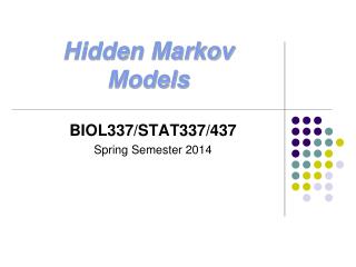
0.94 0.5 0.5 0.91 0.92 0.08 0.06 0.5 0.09 0.5 Expectation-Maximization: Forward-Backward Illustration • Forward-Backward Algorithm, Iteration 2: aij bj(ot) μ σ2 ot , aij P(qt=j|O,) j, j
0.93 0.53 0.75 0.88 0.93 0.07 0.07 0.25 0.12 0.47 Expectation-Maximization: Forward-Backward Illustration • Forward-Backward Algorithm, Iteration 3: aij bj(ot) μ σ2 ot , aij P(qt=j|O,) j, j
0.91 0.58 0.88 0.85 0.93 0.07 0.08 0.12 0.15 0.42 Expectation-Maximization: Forward-Backward Illustration • Forward-Backward Algorithm, Iteration 4: aij bj(ot) μ σ2 ot , aij P(qt=j|O,) j, j
0.89 0.85 0.87 0.78 0.94 0.06 0.11 0.13 0.22 0.15 Expectation-Maximization: Forward-Backward Illustration • Forward-Backward Algorithm, Iteration 10: aij bj(ot) μ σ2 ot , aij P(qt=j|O,) j, j
0.89 0.84 0.87 0.73 0.94 0.06 0.11 0.13 0.27 0.16 Expectation-Maximization: Forward-Backward Illustration • Forward-Backward Algorithm, Iteration 20: aij bj(ot) μ σ2 ot , aij P(qt=j|O,) j, j
Embedded Training • Typically, when training a medium- to large-vocabulary system, each phoneme has its own HMM; these phoneme-level HMMs are then concatenated into a word-level HMM to form the words in the vocabulary. • Typically, forward-backward training is for training the phoneme-level HMMs, and uses a database in which the phonemes have been time-aligned (e.g. TIMIT) so that each phoneme can be trained separately. • The phoneme-level HMMs have been trained to maximize the likelihood of these phoneme models, and so the word-level HMMs created from these phoneme-level HMMs can then be used to then recognize words. • In addition, we can train on sentences (word sequences) in our training corpus using a method called embedded training.
y1 y2 E1 E2 E3 s1 s2 s3 y3 y1 y2 E1 E2 E3 s1 s2 s3 y3 Embedded Training • Initial forward-backward procedure trains on each phoneme individually: • Embedded training concatenates all phonemes in a sentence into one sentence-level HMM, then performs forward-backward training on the entire sentence:
AX TS ER OW L L SH AA ER L AX AA OW SH TS L TS AA SH OW ER L AX L Embedded Training • Example: Perform embedded training on a sentence from the Resource-Management (RM) corpus: • “Show all alerts.” • First, generate phoneme-level pronunciations for each word • Second, take existing phoneme-level HMMs and concatenate them into one sentence-level HMM. • Third, perform forward-backward training on this sentence-level HMM. SHOW ALL ALERTS SH OW AA L AX L ER TS
Embedded Training • Why do embedded training? • Better learning of acoustic characteristics of specific words.(the acoustics of /r/ in “true” and “not rue” are somewhat different, even though the phonetic context is the same) • Given initial phoneme-level HMMs trained using forward-backward, can perform embedded training on muchlarger corpus of target speech using only the word-leveltranscription and a pronunciation dictionary. Resulting HMMs are then (a) trained on more data and (b) tuned to specific words in the target corpus. • Caution: Words spoken in sentences can have pronunciation that is different from the pronunciation obtained from a dictionary. (Word pronunciation can be context-dependent or speaker- dependent).