
Introduction
E N D
Presentation Transcript
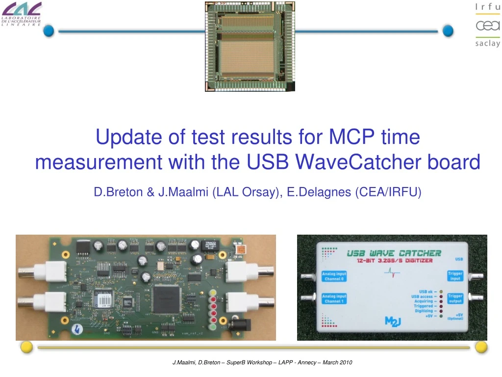
Update of test results for MCP time measurement with the USB WaveCatcher board D.Breton & J.Maalmi (LAL Orsay), E.Delagnes (CEA/IRFU)
Goals of the study : proving the feasibility of using analog memories for characterizing MCP-PMTs on test bench. The complexity of the algorithm used is not an issue finding a simple solution for high range On-Detector electronics The chosen algorithm has to fit easily in a standard FPGA (ProAsic3 from ACTEL) a NIM article in collaboration with SLAC and Hawaii University will soon be published It includes results from both TARGET and WaveCatcher boards. Introduction
The USB_WaveCatcher board The goal of the study is to measure our capacity to perform the measurement of the time difference between two pulses (like a TDC but directly with analog pulses!). Pulsers for reflectometry applications Reference clock: 200MHz => 3.2GS/s 1.5 GHz BW amplifier. Board has to be USB powered => power consumption < 2.5W µ USB Trigger input 2 analog inputs. DC Coupled. Trigger output +5V Jack plug Trigger discriminators Cyclone FPGA SAM Chip Dual 12-bit ADC
Acquisition software with graphical user interface This software can be downloaded on the LAL web site at the following URL: http://electronique.lal.in2p3.fr/echanges/USBWaveCatcher/
Jitter sources • Jitter sources are : • Electronics noise : depends on the design and on the bandwidth of the system • => converts into jitter with the signal slope • Sampling jitter : due to clock Jitter and to mismatches of elements in the delay chain. • => induces dispersion of delay durations • 2.1 Random fluctuations : Random Aperture Jitter(RAJ) • Clock Jitter + Delay Line => depends on design • 2.2 Fixed pattern fluctuations : Fixed Aperture Jitter(FPJ) • => systematic error in the sampling time => can be corrected
Noise Time Time Jitter Jitter induced by electronics noise Simplified approach slope = 2ЛAf3db tr ~ 1/(3 f3db) Zoom Jitter vs Bandwidth and SNR : Jitter [ps] ~ Noise[mV] / Signal Slope [mV/ps] ~ tr / SNR Ex: the slope of a 100mV - 500MHz sinewave gets a jitter of ~2ps rms from a noise of 0.6mV rms • Conclusions: • The higher the SNR, the better for the measurement • As the maximum slope of the signal is proportional to the measurement system bandwidth and as the noise is only proportional to its square root, a higher bandwidth favours a higher time precision (goes with its square root). • But: for a given signal, it is necessary to adapt the bandwidth of the measurement system to that of the signal in order to keep the noise-correlated jitter as low as possible • Problems occur with ultra fast signals with a bandwidth > 1GHz …
Fake signal Δt[cell] Real signal After interpolation Effects of the Fixed Pattern Jitter • Dispersion of single delays => time DNL • Cumulative effect => time INL. Gets worse with delay line length • Systematic effect => non equidistant samples (bad for FFT). • If we can measure it, we can correct it ! In a Matrix system, DNL is mainly due to signal splitting into lines => modulo 16 pattern • => correction with Lagrange polynomial interpolation. Drawbacks: computing power. • => good (and easy) calibration required.
Open cable USB Wave Catcher USB Wave Catcher Measurement : Time distance beween two pulses Two pulses on different channels Two pulses on the same channel => with this setup, we can measure precisely the time difference between the pulses independently of the timing characteristics of the generator!
Measurement results for time distance • Source: asynchronous set of two positive pulses • Time difference between the two pulses extracted by crossing of a fixed threshold determined by polynomial interpolation of the 4 neighboring points (on 3000 events). Vth
Jitter vs Time distance between two pulses Source: asynchronous set of two positive pulses Results are the same with negative pulses or distance between arches of a sine wave Jitter distribution after INL correction is almost flat => coherent with INL shape
Chi-square method Goal : Measuring the time difference between pulses coming from the two MCP-PMTs. Chi2 is a complexmethod but issupposed to be the most precise method for time measurement Description : Spline interpolation between samples Data normalization Data alignment ( on Peak or on a Constant fraction) Computing of the average pulse for each channel Sliding of the average pulses across each individual pulse : search for the time that minimizes the sum of the squared difference between the two shapes (we can use only the leading edge).
Results from first data taking (5000 events) 600 raw pulses aligned on amplitude (spline interpolation between samples)
600 normalized pulses superimposed Common threshold
Average pulse and 2- σ templates « Average » pulse: black Average +/-2 σ: red
Results with Chi-Square Method chi2 method using reference pulse between 10% and 35% Double Pulse resolution: σ = 23.4ps rms (no gaussian fit) => single : ~ 16,7 ps σ =22.7ps (gaussian fit) => single : ~ 16,2 ps
Why a Constant Fraction discriminator (CFD) ? A simple threshold method introduces aTime Walk that depends on the signal amplitude! Digital CFD Method Threshold is a constant fraction of the amplitude Fixed threshold Δt Δt ~ 0 • Differentmethods have been compared : • Spline Interpolation to find the maximum + Spline Interpolation to findthreshold. • Spline interpolation for the maximum + Linear interpolation for the threshold • No interpolation for the maximum+ Linear interpolation for the thresholdcrossing • No interpolation for the maximum + Spline Interpolation for the threshold
Digital CFD results : Fraction ratio = 23%. Double Pulse resolution: σ(ΔT) = 23.4ps rms ( no gaussian fit) σ (ΔT)=23ps (with a gaussian fit) Nearlyindependent on fraction ratio in the 0.25-0.5 range
Results with CFD Method Conclusion : From this we could conclude that applying a very simple algorithm, which is very simple to integrate in a FPGA (finding a maximum & linear interpolation between two samples, i.e., without a use of the Spline fit) already gives very good results (only 10% higher than the best possible resolution limit).
NIM paper is on its way There is a considerable interest to develop new time-of-flight detectors using, for example, micro-channel-plate detectors (MCP-PMTs). The question we posed in this paper is if the new waveform digitizers, such as the Wave Catcher and TARGET ASIC chips, operating with a sampling rate of 2-3 GSa/s can compete with a 1GHz BW CFD/TDC/ADC electronics. ... Although the commercial CFD-based electronics does exist and performs very well, it is difficult to implement it on a very large scale, and therefore the custom electronics has to be designed. In addition, the need of analog delay line makes it very difficult to incorporate the CFD discriminator in the ASIC designs.
Conclusion • The USB Wave Catcher has become a nice demonstrator for the use of matrix analog memories in the field of ps time measurement • During the last one and a half year, we have learned a lot about the optimization of both analog memories and board design for time measurement • Different methods have been studied to analyze data taken with MCP-PMTs : • CFD and Chi2 algorithm give almost the same time resolution : • Double pulse resolution ~ 24 ps => Single pulse resolution ~ 17 ps • Event the simplest CFD algorithm can give a good timing resolution • Single pulse resolution ~ 18 ps • it can be easily implemented inside an FPGA (our next step) • => reduces the data rate => can be used for very large scale detectors
Summary of the board performances. • 2 DC-coupled 256-deep channels with 50-Ohm active input impedance • ±1.25V dynamic Range, with full range 16-bit individual tunable offsets • 2 individual pulse generators for test and reflectometry applications. • On-board charge integration calculation. • Bandwidth > 500MHz • Signal/noise ratio: 11.9 bits rms • (noise = 630 µV RMS) • Sampling Frequency: 400MS/s to 3.2GS/s • Max consumption on +5V: 0.5A • Absolute time precision in a channel (typical): • without INL calibration: 16ps rms (3.2GS/s) • after INL calibration <10ps rms (3.2GS/s) • Relative time precision between channels: <5ps rms. • Trigger source: software, external, internal, threshold on signals • Acquisition rate (full events) Up to ~1.5 kHz over 2 full channels • Acquisition rate (charge mode) Up to ~40 kHz over 2 channels


