Introduction to SPC
400 likes | 790 Vues
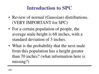
Introduction to SPC. Review of normal (Gaussian) distributions. (VERY IMPORTANT for SPC) For a certain population of people, the average male height is 68 inches, with a standard deviation of 3 inches.

Introduction to SPC
E N D
Presentation Transcript
Introduction to SPC • Review of normal (Gaussian) distributions. (VERY IMPORTANT for SPC) • For a certain population of people, the average male height is 68 inches, with a standard deviation of 3 inches. • What is the probability that the next male from this population has a height greater than 70 inches? (what information here is missing?)
Normal Review (continued) • What is the probability that the average height of the next nine males is greater than 70 inches? • Central Limit Theorem (see next slide) • If the mean of the population shifted to 72 inches, what is the probability that the next male is less than 70 inches (assume normal distribution)? • If a sample of nine came from the new population, what is the probability the average of the sample will be less than 70 inches?
Central Limit Theorem: Example of the Roll of the Dice Theoretical Frequency Distribution based on 216 rolls... Average of Two Dice m=3.5, s=1.23 Average of Three Dice m=3.5, s=0.99 One Die m=3.5, s=1.87
Customer Supplier Statistical Process Control • Sample output of process and • make inferences about its state • Demonstrate that the • distribution of process output • is known and unchanging • Plot and monitor over time • Use statistical tests to detect shifts • and anomalies and react to them quickly • Use statistical evidence to guide and • confirm process improvements
100% Insp. 100% Insp. Supplier Customer Supplier Customer Supplier Supplier Customer Customer 100% Insp. Sample Insp. Sample Insp. Evolution from Inspection to SPC SPC. SPC. SPC.
Statistical Process Control Topics • Introduction to Variability • Control Charts • General info • x-bar Charts, R Charts • p Charts, np Charts • Type 1 and Type 2 Errors • Process Capability Analysis
Measure Performance Variation “The less variation, the better off we are.” Improve Capabilities Common cause variation: Inherent in the system Assignable cause variation: Event-related, special (assignable ~ special) Analyze and Act
Analyze and Act: React to Assignable Causes • Note unusual variation diagnosed by using a common test to evaluate individual data points • Identify cause by noting what change in the process occurred at that point in time • Eliminate cause or build in the cause • Monitor performance to verify the effect of the “fix” • Generally, assignable causes cause points outside of control limits!
Improve Process Capabilities: Drive Out Common Causes • Variation is inherent in the system • Don’t react to individual points (this is tampering) • Analyze possible factors affecting variation (use Cause and Effect Diagram, Pareto Analysis) • Work to reduce variation: Make an improvement, that is, introduce a special cause • Monitor performance to verify the effect of the intended improvement
Customer Supplier X-bar and R charts • Sample output of process - parameter • of interest is continuously variable • Plot one chart to track sample means and • another one to track sample ranges (variation) • Use statistical evidence to detect changes • and improve the process: to better position • the mean and to reduce variation
Underlying Assumptions • process mean m and standard deviation s when the process is in control • process may go out of control in two possible ways • mean shifts to m1, with standard deviation unchanged • standard deviation shifts to s1, with mean unchanged • sample means are normally distributed (when in or out of control, because either: • process output measurements on individual units are normally distributed when in or out of control • OR Central Limit Theorem applies: • n > 30 OR • If distribution unimodal or symmetric, then much smaller n’s are acceptable to assume normality (n on the order of 4).
Basic Probabilities Concerning the Distribution of Sample Means Std. dev. of the sample means:
Estimation of Mean and Std. Dev. of the Underlying Process • use historical data taken from the process when it was “known” to be in control • usually data is in the form of samples (preferably with fixed sample size) taken at regular intervals • process mean m estimated as the average of the sample means (the grand mean) • process standard deviation s estimated by: • standard deviation of all individual samples • OR mean of sample range R/d2, where sample range R = max. in sample minus min. in sample and d2 = value from look-up table (appendix A-7)
Output Sample Sample Measurements Mean Range 1 2 2 3 4 2 2.6 2 2 2 4 2 1 2 2.2 3 3 1 2 4 1 2 2.0 3 4 2 2 3 4 2 2.6 2 5 2 1 2 3 1 1.8 2 6 1 5 2 2 3 2.6 4 Average: m=2.3 R=2.7 Sample Example: Estimation of Mean and Std. Dev. of the Underlying Process Estimate of the process mean = m = 2.3 Estimate of the process std. dev.: (1) Combined std. dev. of all 30 points: s = 1.1 OR (2) s = R/d2 (n=5) = 2.7/2.326 = 1.2
Determination of Control Limits For the x-bar chart: - Center Line = grand mean - Control Limits: Co's usually use - Can analyze process capability based on the specification limits For the R chart: - Center Line = average range = - Control Limits: Alternative: Use an Economic Approach: - Consider the cost impact of out-of-control detection delay (Type 2 error), false alarm (Type 1 error) and sampling costs - Difficult to estimate costs
Ex. Two Machines -Process Capability Analysis and x-bar and R-charts
X-bar vs. R charts • R charts monitor variability: Is the variability of the process stable over time? Do the items come from one distribution? • X-bar charts monitor centering (once the R chart is in control): Is the mean stable over time? >> Bring the R-chart under control, then look at the x-bar chart
How to Construct a Control Chart 1. Take samples and measure them. 2. For each subgroup, calculate the sample average and range. 3. Set trial center line and control limits. 4. Plot the R chart. Remove out-of-control points and revise control limits. 5. Plot x-bar chart. Remove out-of-control points and revise control limits. 6. Implement - sample and plot points at standard intervals. Monitor the chart.
X-bar and R chart example: • Look at handout: R Chart. • R-bar = sum( R )/num. samples = 87/25 = 3.48. • UCL = D4R-bar = 2.114*3.48 = 7.357. • LCL = D3R-bar = 0 • Review samples, eliminate sample 3. • Do over! New R-bar = 3.29, UCL = 6.95 • R-bar chart now in control, proceed to X-bar!
X-bar chart • Grand mean, X-bar = 500.6/24 = 20.86. • Control limits = 20.86 +/- A2R-bar = 20.86 +- (.5777)*3.29 • UCL = 20.86 + 1.9 = 22.76 • LCL = 20.86 – 1.9 = 18.96 • Bring X-bar chart under control—eliminate points 15, 22, 23.
Conclusion of problem Redo R chart without samples 15, 22, and 23 (and 3 is out as well). R-bar = 3.24 Control limits (repeat previous procedure = [0, 6.845]. Grand mean (center line for x-bar) = 20.77 Control limits = 20.77 +/- (.5777)(3.24) = [18.90, 22.64] Our control limits for both charts are now set.
Alarm No Alarm In-Control Out-of-Control Type 1 and Type 2 Error
Common Tests to Determine if the Process is Out of Control • One point outside of either control limit • 2 out of 3 points beyond UCL - 2 sigma • 7 successive points on same side of the central line • of 11 successive points, at least 10 on the same side of the central line • of 20 successive points, at least 16 on the same side of the central line
Type 1 Errors for these Tests Test Probability Type 1 Error 1/1 2(0.00135) 0.0027 2/3 0.00052 7/7 (0.5)7 0.0078 10/11 0.00586 16/20 0.0059
Type 2 Error Suppose m1 > m Type 2 Error = • [This is the probability of a sample average being below the upper control limit. We have not examined possibility of being below LCL, why?] • Power = 1- Type 2 Error. Power increases as … • n increases, as (m1-m) increases, and as s decreases. • Extension to m1 < m is straightforward
Sensitivity of Type I and Type II Errors • To (UCL-LCL)/s • To n • To s • To m1 - m
Example of Type 1 and 2 Errors Suppose: m = 100 m1= 102 s = 4 n = 9 [assume 3 sigma control limits] Find Type 2 Error:
Example of Type 1 and 2 Errors (cont.) Type 2 Error = Type 1 Error = Prob{Shift detected in third sample after shift occurred} = Average number of samples taken before the shift is detected = Prob{no false alarm for first 32 samples, but then false alarm occurs in 33rd sample} Average number of samples before a false alarm (ARL)