Static Huffman
Static Huffman. A known tree is used for compressing a file. A different tree can be used for each type of file. For example a different tree for an English text and a different tree for a Hebrew text. Two passes on file. One pass for building the tree and one for compression.

Static Huffman
E N D
Presentation Transcript
Static Huffman • A known tree is used for compressing a file. • A different tree can be used for each type of file. For example a different tree for an English text and a different tree for a Hebrew text. • Two passes on file. One pass for building the tree and one for compression. 3. 1
Wrong probabilities • What is different in this text? 3. 2
Adaptive Huffman • xt is encoded with tree of x1,...,xt-1. • Tree is changed during compression. • Only one pass. • No need to transmit the tree. • Two possibilities: • At the beginning assume each item appeared once. • At the beginning probabilities are wrong but after a large amount of data the error is negligible. • When a new character appears send an escape character before it. 3. 3
Algorithm for canonical trees • Find a Huffman tree with lengths L1,...,Ln for the items. • Sort the items according to their lengths. • Assign to each item the first Li bits after the binary point of 3. 5
Example of a canonical tree • Suppose the lengths are: • A-3, B-2, C-4, D-2, E-3, F-3, G-4 • The sorted list is: • B-2, D-2, A-3, E-3, F-3, C-4, G-4 3. 6
Why canonical trees? • A canonical tree can be transferred easily. • Send number of items for every length. • Send order of items. • Canonical codes synchronize faster after errors. • Canonical codes can be decoded faster. 3. 7
Errors in Huffman coded files • In the beginning God created the heaven and the earth. And the earth was without form, and void; and darkness was upon the face of the deep. And the Spirit of God moved upon the face of the waters. And God said, Let there be light: and there was light. And God saw the light, that it was good: and God divided the light from the darkness. And God called the light Day, and the darkness he called Night. And the evening and the morning were the first day. And God said, Let there be a firmament in the midst of the waters, and let it divide the waters from the waters... • What will happen if the compressed file is read from arbitrary points? • : ac darkness was upon the face • csoaraters. And God said, Let there be light • d lnrathat it was good: and God divided • .aauya dy, and the darkness he called Night • c y. And God said, Let there be a firmament in the midst 3. 8
erroneous synchronization correct erroneous synchronization correct Synchronization after error • If the code is not an affix code: 3. 9
Definitions • Let P1,...,Pn be the probabilities of the items (The leaves of the Huffman tree). • Let L1,..,Lnbe the length of codewords. • Let X be the set of internal nodes in the Huffman tree. • xXlet Ix be the set of leaves in the sub-tree rooted by x. 3. 10
Formulas • Average codeword's length is • The Probability that an arbitrary point in the file will be in node x is: • xX and yIx define: • Q(x,y)= { • if the path from x to y corresponds to a sequence of one or more codewords in the code 0 otherwise 3. 11
Synchronization's probability • Let S denote the event that the synchronization point is at the end of the codeword including xX. 3. 12
Probability for a canonical tree • Nelson's trees are the trees described in 2.2 with some other features. 3. 13
Synchronization • canonical trees synchronize better since every sub-tree of a canonical tree is a canonical tree itself. • Expected number of bits until synchronization is: 3. 14
Expected synchronization 3. 15
0 000 1 0010 2 0011 3 0100 4 01010 5 01011 6 01100 7 01101 8 011100 9 011101 10 011110 11 011111 12 100000 13 100001 14 100010 15 100011 16 1001000 17 1001001 18 1001010 ... 29 1010101 30 1010110 31 10101110 32 10101111 ... 62 11001101 63 110011100 64 110011101 ... 125 111011010 126 1110110110 127 1110110111 ... 199 1111111111 Skeleton Trees • No need to save the whole tree e.g. if a codeword starts with 1101, it ought to be of length 9 bits. Thus, we can read the following 5 bits as a block. 3. 16
Illustration of a Skeleton Tree • This is the skeleton tree for the code on the previous slide. It has 49 nodes, while the original one has 399 nodes. 3. 17
Definition • Let m=min{ l | ni>0 } where nl is the number of codewords of length l. • Let base(l) be: • base(m)=0 • base(l)=2(base(l-1)+nl-1) • Let seq(l) be: • seq(m)=0 • seq(l)=seq(l-1)+nl-1 3. 18
Definition (cont.) • Let Bs(k) denote the s-bit binary representation of the integer k with leading zeros if necessary. • Let I(w) be the integer value of the binary string w, i.e. if w is of length of l, w=Bl(I(w)). • I(w)-base(l) is the relative index of codeword w within the block of codewords of length l. • seq(l)+I(w)-base(l) is the relative index of w within the full list of codewords. This can be rewritten as I(w)-diff(l), for diff(l)=base(l)-seq(l). • Thus all one needs is the list of diff(l). 3. 19
An example for values • These are the values for the code depicted on the previous slides. 3. 20
Decoding Algorithm • tree_pointerroot • i1 • start1 • while i<length_of_string • if string[i]=0 tree_pointerleft(tree_pointer) • else tree_pointerright(tree_pointer) • if value(tree_pointer)>0 • codewordstring[start…(start+value(tree_pointer)-1)] • outputtable[I(codeword)-diff[value(tree_pointer)]] • tree_pointerroot • startstart+value(tree_pointer) • istart • else i++ 3. 21
Reduced Skeleton Trees • Define for each node v of the Skeleton Tree: • If v is a leaf • lower(v)=upper(v)=value(v) • If v is an internal node • lower(v)=lower(left(v)) • upper(v)=upper(right(v)) • Reduced Skeleton Tree is the smallest sub-tree of the original Skeleton Tree for which all the leaves w hold: • upper(w)lower(w)+1 3. 22
Illustration of a reduced tree • This is the reduced tree of the previous depicted tree. • If 111 have been read we can know that the length of the codeword is either 9 or 10. • If the bits after 111 were 0110, we would have performed four more comparisons and still cannot know if the length is 9 or 10 3. 23
Another example of a reduced tree 5 00000 6 010001 7 0101111 8 10011101 9 110010011 10 1110100101 11 11110111111 12 111111010101 13 1111111011111 • This is a reduced Skeleton Tree for bigrams of the Hebrew Bible. Just lengths up to 13 are listed. 3. 24
Algorithm of reduced trees • tree_pointerroot • istart1 • while i<length_of_string • if string[i]=0 tree_pointerleft(tree_pointer) • else tree_pointerright(tree_pointer) • if value(tree_pointer)>0 • lenvalue(tree_pointer) • codewordstring[start…(start+len-1)] • if flag(tree_pointer)=1 and 2I(codeword)base(len+1) • codewordstring[start...(start+len) • len++ • outputtable[I(codeword)-diff[len]] • tree_pointerroot • istartstart+len • else i++ 3. 25
Affix codes • Affix codes are never synchronizing, but they can be decoded backward. • PL/1 allows files on magnetic tapes to be accessed in reverse order. • Information Retrieval systems use concordance points to the words’ locations in the text. When a word is retrieved, typically, a context of some words is displayed. 3. 26
Non-Trivial Affix codes • Fixed length codes are called trivial affix codes. • Theorem: There are infinite non-trivial complete affix codes. • Proof: One non-trivial code is showed in this slide. Let A={a1,...,an} be an affix code. Consider the set B={b1,...,b2n} defined by b2i=ai0, b2i-1=ai1 for 1in. Obviously B is an affix code. 01 000 100 110 111 0010 0011 1010 1011 3. 27
Markov chains • A sequence of events, each of which depends only on n events before it, is called an nth Order Markov chain. • First order Markov chain - Event t is depending just on event t-1. • 0th order Markov chain - events are independent. • Examples: • Fibonacci sequence is a second order chain. • An arithmetic sequence is a first order chain. 3. 28
Markov chain of Huffman trees • A different Huffman tree for each item in the set. • The tree for an item x will have the probabilities of each item to appear after x. • Examples: • u will have a much shorter codeword in q's tree, than other trees. • ט will have a much longer codeword after ג. • This method implements a first order Markov chain. 3. 29
Clustering • Markov chains for Huffman trees can be expanded for nth order chains. • Overhead for saving so many trees can be very high. • Similar trees can be clustered into a one tree, which will be the average of the original trees. • Example: The trees of v and b may be similar since they have a similar sound. 3. 30