Download
1 / 9
110 likes | 755 Vues
The Bellman-Ford Shortest Path Algorithm Neil Tang 03/11/2010. Class Overview. The shortest path problem Differences The Bellman-Ford algorithm Time complexity. Shortest Path Problem. Weighted path length (cost): The sum of the weights of all links on the path.

E N D
The Bellman-Ford Shortest Path Algorithm Neil Tang03/11/2010 CS223 Advanced Data Structures and Algorithms
Class Overview • The shortest path problem • Differences • The Bellman-Ford algorithm • Time complexity CS223 Advanced Data Structures and Algorithms
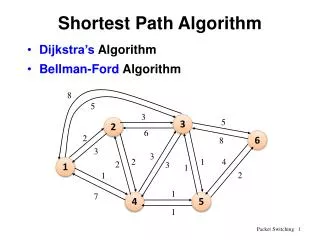
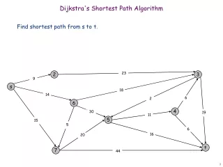
Shortest Path Problem • Weighted path length (cost): The sum of the weights of all links on the path. • The single-source shortest path problem: Given a weighted graph G and a source vertex s, find the shortest (minimum cost) path from s to every other vertex in G. CS223 Advanced Data Structures and Algorithms
Differences • Negative link weight: The Bellman-Ford algorithm works; Dijkstra’s algorithm doesn’t. • Distributed implementation: The Bellman-Ford algorithm can be easily implemented in a distributed way. Dijkstra’s algorithm cannot. • Time complexity: The Bellman-Ford algorithm is higher than Dijkstra’s algorithm. CS223 Advanced Data Structures and Algorithms
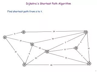
x t 5 ,nil ,nil 6 -2 -3 0 8 s -4 7 2 7 ,nil ,nil 9 z y The Bellman-Ford Algorithm CS223 Advanced Data Structures and Algorithms
x x x x t t t t 5 5 5 5 2,x 6,s ,nil 6,s ,nil 4,y 4,y ,nil 6 6 6 6 -2 -2 -2 -2 -3 -3 -3 -3 0 0 0 0 8 8 8 8 s s s s -4 -4 -4 -4 7 7 7 7 2 2 2 2 7 7 7 7 ,nil 7,s 7,s 7,s ,nil ,nil 2,t 2,t 9 9 9 9 z z z z y y y y The Bellman-Ford Algorithm Initialization After pass 1 After pass 2 After pass 3 The order of edges examined in each pass:(t, x), (t, z), (x, t), (y, x), (y, t), (y, z), (z, x), (z, s), (s, t), (s, y) CS223 Advanced Data Structures and Algorithms
x t 5 2,x 4,y 6 -2 -3 0 8 s -4 7 2 7 7,s -2,t 9 z y The Bellman-Ford Algorithm After pass 4 The order of edges examined in each pass:(t, x), (t, z), (x, t), (y, x), (y, t), (y, z), (z, x), (z, s), (s, t), (s, y) CS223 Advanced Data Structures and Algorithms
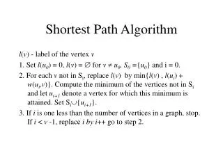
The Bellman-Ford Algorithm Bellman-Ford(G, w, s) Initialize-Single-Source(G, s) for i := 1 to |V| - 1 do for each edge (u, v) E do Relax(u, v, w) for each vertex v u.adj do if d[v] > d[u] + w(u, v) then return False // there is a negative cycle return True • Relax(u, v, w) • if d[v] > d[u] + w(u, v) • then d[v] := d[u] + w(u, v) • parent[v] := u CS223 Advanced Data Structures and Algorithms
Time Complexity Bellman-Ford(G, w, s) Initialize-Single-Source(G, s) for i := 1 to |V| - 1 do for each edge (u, v) E do Relax(u, v, w) for each vertex v u.adj do if d[v] > d[u] + w(u, v) then return False // there is a negative cycle return True O(|V|) O(|V||E|) O(|E|) Time complexity: O(|V||E|) CS223 Advanced Data Structures and Algorithms