Download
1 / 37
380 likes | 630 Vues
Soil Moisture Data Assimilation in the SHEELS Land Surface Model. Clay Blankenship USRA Special thanks to: Bill Crosson, Jon Case. Overview. Data assimilation and retrieval background 1dvar, 3dvar, and Kalman Filters Soil Moisture Data Assimilation SHEELS LSM AMSR-E data Results

E N D
Soil Moisture Data Assimilation in the SHEELS Land Surface Model Clay Blankenship USRA Special thanks to: Bill Crosson, Jon Case
Overview • Data assimilation and retrieval background • 1dvar, 3dvar, and Kalman Filters • Soil Moisture Data Assimilation • SHEELS LSM • AMSR-E data • Results • Some results from profile retrievals with MIRS
Data Assimilation (and Variational Retrievals) Given observations {y} and background state {xb}, estimate most likely state {x} taking into account errors in both xb and y. P(UT fan|orange shirt)=P(orange shirt|UT fan)P(UT fan) P(orange shirt) { { Retrieved-Bkgd State Obs-Calc Obs x: geophysical state xb: background (a priori) of state y: observations H(x): forward operator converting x into observation space Pb: background error covariance R: obs+forward model error covariance • In “data assimilation” you are using observations to improve a model. In “profile retrievals” you always have some assumed background state (maybe climatology).
Data Assimilation (and Variational Retrievals) Given observations {y} and background state {xb}, estimate most likely state {x} taking into account errors in both xb and y. To maximixe this probability, minimize -2 times its log: Bkgd Error Cov O+F Error Cov { { Retrieved-Bkgd Atmosphere Obs-Calc TB
DA Solution simplified: Minimizing the cost function: Given initial guess x=xb, linearize and solve for new estimate of x. Skipping the math, the solution can be expressed as: The “Gain” represents a weighted average of bk and ob errors The Jacobian K relates the y terms to x terms and can include interpolation, averaging or integration, radiative transfer, etc. Bkgd Gain Innovation
Data Assimilation Methods Hybrid methods use ensemble spread to define background covariance in 3dvar.
Soil Moisture Data Assimilation in the SHEELS Land Surface Model
SHEELS – Simulator for Hydrology and Energy Exchange at the Land Surface SHEELS • Distributed land surface hydrology model provides soil state(T,q), fluxes of energy and moisture • Heritage: 1980’s Biosphere-Atmosphere Transfer Scheme (BATS) • Can run off-line or coupled with meteorological model • Flexible vertical layer configuration designed to facilitate microwave data assimilation • Described in Martinez et al. (2001), Crosson et al. (2002)
SHEELS Input SHEELS Input • Required static variables: • Soil type (STATSGO):Landcover (U of Md): • Saturated hydraulic conductivity Canopy height • Saturated matric potential Fractional vegetation cover • Soil wilting point Minimum stomatal resistance • Soil porosity Root depth • Reflectance properties • Seasonal: • Leaf area index Topography (GTOPO30): • Surface elevation and slope • Time-dependent input (forcing): • Wind speed (NLDAS) • Air temperature • Relative humidity • Atmospheric pressure • Downwelling solar radiation • Downwelling longwave radiation • Rainfall (Stage IV)
SHEELS Output STATES Soil surface and canopy temperatures Soil temperature Soil water/ice content Depth of water on canopy Ponded water Snow temperature, depth, and density FLUXES Surface latent and sensible heat fluxes Ground heat flux Net radiation flux Evapotranspiration Infiltration Runoff
Land Information System (LIS) A modeling and data assimilation system with the capability to run several different LSMs, from GSFC’s Hydrological Sciences Branch. It is very customizable with the ability to swap out LSMs, forcing datasets, etc. LSMS VIC, Noah, CLM, Catchment,SiB2, Hyssib Base Forcings ECMWF, GDAS, NLDAS... Supplemental Forcings TRMM 3B42, Agrrad, Cmap, Cmorph, Stg4... Parameters Landcover, soils, greenness, albedo, LAI, topography, tbot Data Assimilation algorithm, observation, perturbation method
Example Depth-Time Sections NebraskaJAN-JUL 2003 Fractional soil moisture (water+ice) Soil Temperature
SHEELS output time series SHEELS output time series Volumetric soil moisture, 1 Mar 2011 - 21 Apr 2011 0-10cm Root zone Total column (10m) Salinas, California 14
AMSR-E (Advanced Microwave Scanning Radiometer for EOS) AMSR-E retrieved soil moisture for August 2, 2008 over the SE US NASA Aqua satellite with AMSR-E instrument AMSR-E • Conically scanning passive microwave radiometer on NASA Aqua polar orbiter • Measures polarized brightness temperatures at 6 frequencies from 6.9 to 89.0 GHz • We use the Level 3 retrieved soil moisture product (Njoku et al. 2003) resampled to a 25-km grid. (Obs twice daily.) • Stated accuracy is .06 m3/m3. (Typical range is .05 to .40) • Algorithm minimizes differences between the observed brightness temperatures and those generated using a forward radiative transfer model. • Due to extensive radio frequency interference in the 6.9 GHZ channel, 10.7 and 18.7 GHz observations are used for soil moisture estimation.
Background and Observed Variables q1 q2 • SHEELS state variables (x) include temperature and fractional water content in each of 14 layers • 6 in the top 10 cm • 6 root zone (up to 1.5m) • 2 deep layers to 10m. The observation* (y) (retrieved soil moisture) is the volumetric water content (cm3/cm3) near the surface (exponentially weighted by depth) Mostly top layer but must account for porosity to convert from FWC to VWC *Actually a retrieval or estimate but in the context of data assimilation it’s an observation. q3 q4 q5 q6 q7 q8 q9
The ensemble consists of N model state fields. • The mean of the N ensemble states is used to define the state vector estimate. • The spread of an ensemble of N model ‘trajectories’ is used to estimate the error covariances. The full non-linear dynamic equations are used to propagate each ensemble member forward in time, thus determining the trajectories. This is in contrast to the traditional Kalman filter in which linearized model dynamics are used to propagate error covariances. • When observations are available, each ensemble member is updated based on the difference between the observation and the model state, weighted by the Kalman gain (as in the EKF). • Random error is added to the observation based on assumed noise characteristics; this ensures that the variance of the updated ensemble matches the true estimation error covariances (Burgers et al., 1998, Mon. Wea. Rev.) • Propagation of error covariance matrix is more stable than in the traditional Kalman filter, especially if there are strong non-linearities in the model. Ensemble Kalman Filter in LIS
Micronet Validation • First validation attempt vs. ARS Micronet (Little Washita River, OK) • Large bias and variability due to sampling error and soil properties • Ran artificial experiments with 0.5x and 1.5x rain forcing, validated against Micronet and “truth” run. • Large errors remain, but DA runs (dashed) tend to converge • Square-wave error maybe due to day-night bias differences
Bias Correction (CDF Matching) 0.5 0.4 0.3 0.2 0.1 0.0 CDF-Corrected Soil Moisture 0.0 0.1 0.2 0.3 0.4 AMSR-E Observed Soil Moisture AMSR-E Bias Correction The dynamic range of AMSR-E observed soil moisture is small relative to that of the model. A correction (right) is applied to convert the observation into a model-equivalent value. A Cumulative Distribution Function (CDF)-matching technique is used here. This is similar in purpose to the bias corrections usually applied to satellite observations in NWP models. Simulations made without the proper correction showed a pronounced dry bias.
Impact of Land Use CDF CorrectionDifference in fractional soil moisture immediately following assimilation of AMSR-E data at 8 UTC on June 7, 2003: Land Use CDF minus Uniform CDF simulation. The spatial pattern reflects the land use type distribution and illustrates the impact of the Land Use CDF correction on soil moisture data assimilation.
No Rain Experiment 22Z 24 Jun 2003 The data assimilation adds soil water, particularly in the eastern part of the domain and the Texas panhandle. “Truth” Stage IV Precipitation Forcing Control No Data Assimilation Data Assimilation (Combined Bias Correction)
False Rain Experiment 09Z 22 Jun 2003 The data assimilation is able to reduce the water content from the false rainfall in Kansas while increasing it in the Texas panhandle. “Truth” Stage IV Precipitation Forcing Control No Data Assimilation Data Assimilation (Combined Bias Correction)
No Rain Experiment Time series of top layer soil water in SE Nebraska (point marked by diamond at left). The 3 DA runs are able to match the “true” run closely throughout much of the experiment, although they overestimate soil moisture from about June 7-14.
False Rain Experiment Time series of top layer (1.6 cm) soil water fraction from 5 runs (false rain scenario) in Texas panhandle (100.5W, 35N). The DA run with the combined bias correction (red line) shows transitions that are less abrupt (reduced amplitude) during data assimilation steps, compared to the other DA runs (blue/green).
Summary • AMSR-E Soil Moisture Estimates assimilated into SHEELS LSM using EnKF • Bias correction is necessary for good results. • Must be regionally and seasonally appropriate. • Landcover- and day/night-dependent corrections implemented. • Day/night correction alleviates square wave pattern in biases • With hiqh quality forcing data, validation vs. ground truth is difficult • Variability of rainfall and soil properties within a FOV confound this. • Could use anomaly correlations for verification • DA improves modeled soil moisture in simulations with intentionally poor rain forcing • Potentially of greatest use in areas without high-quality continuous rainfall data (radar, gauge networks). • An advantage over microwave (polar orbiting) rainfall observations: It can see the effects of rainfall after it happens (alleviates sampling issue)
Possible Future Work • Validation against ground stations by anomaly correlation • Test impact on a coupled weather forecast model. • Implement for SMOS and SMAP. • AMSR-E .06 cm3/cm3 accuracy • SMOS (ESA, 2009) .04 cm3/cm3 • SMAP (NASA, 2014) .04 cm3/cm3
Microwave Integrated Retrieval System (MIRS) • NOAA STAR algorithm/software package • 1DVAR physically-based retrieval algorithm based on OI theory • Simultaneous retrieval of temperature, humidity, and hydrometeor profiles in EOF space • Water vapor and hydrometeors are in logarithmic coordinates • Assumes local linearity and gaussian pdf of state variable • Applicable to any sensor combining imaging /sounding capabilities. • Experimental products of cloud / precipitation liquid and ice have potential for refinement into contributions to GPM. • Emissivity spectrum is part of the retrieved state vector enabling more direct response to precipitation over land.
MIRS VariablesBackground+3 EOF’s Water Vapor Graupel Cloud Liquid Rain
Intercomparison of AMSU and TRMM Rain Retrievals • Retrievals from AMSU have consistently smaller Rain/Ice amounts compared to TMI • Are these differences due to sensors or algorithms? • Test whether improved first guess and background/covariance constraints can give more consistent results • TRMM and GPM (will) have high resolution measurements but AMSU’s are important for sampling TS Lee (Sep 2, 2011)
MIRS Experiments Sep 2009 Study
MIRS Results (Graupel and Rain) W.Pac. SE US C. Africa • More frequent large ice consistent with high lightning frequency over Africa. • Strong convection, dry environment. MIRS Graupel MIRS Rain