Download
1 / 36
360 likes | 530 Vues
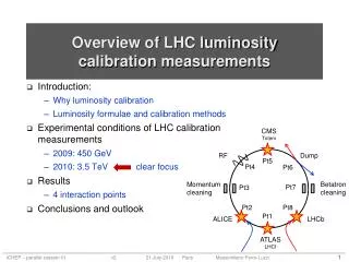
CMS Totem. Overview of LHC luminosity calibration measurements. RF. Dump. Pt5. Pt4. Pt6. Momentum cleaning. Betatron cleaning. Pt7. Pt3. Introduction: Why luminosity calibration Luminosity formulae and calibration methods Experimental conditions of LHC calibration measurements

E N D
CMS Totem Overview of LHC luminosity calibration measurements RF Dump Pt5 Pt4 Pt6 Momentum cleaning Betatron cleaning Pt7 Pt3 Introduction: Why luminosity calibration Luminosity formulae and calibration methods Experimental conditions of LHC calibration measurements 2009: 450 GeV 2010: 3.5 TeV clear focus Results 4 interaction points Conclusions and outlook Pt2 Pt8 Pt1 ALICE LHCb ATLAS LHCf
Acknowledgements Many thanks to • ALICE Collaboration • ATLAS Collaboration • CMS Collaboration • LHCb Collaboration • LHC machine groups
Direct luminosity determination Will focus here on the two methods used at LHC: • Van der Meer method • based on beam separation scans • Beam-gas imaging method • based on beam-gas vertex reconstruction
Why luminosity determination is important Rate = Luminosity x Cross section • Allows to determine cross section of interaction processes on an absolute scale • At the LHC: Heavy flavour production, couplings of new particles, total (inelastic, elastic) cross section, … • Allows to quantify the performance of the collider • Important to verify experimental conditions, to understand quantitatively beam-beam effects, …
Chronology 2009 • All experiments started off with a normalisation based on a generator model including detector simulation => uncertainties at the level of 20% for 450 GeV • LHCb performed first direct luminosity normalisation at 450 GeV using the beam-gas imaging method (see later) 2010 • At 3.5 TeV, started off again with a normalisation based on a generator model including detector simulation • Then, April-May, performed first direct luminosity measurement at each IP with van der Meer scans (+continuous beam-gas imaging normalisation, LHCb)
Van der Meer’s trick See Ref. [1] Consider single circulating & colliding bunch pair with zero crossing angle R = L = f N1 N2 1(x,y) 2(x,y) dx dy With transverse displacements x , y of one beam w.r.t. the other: R (x , y) = L(x , y) = f N1 N2 1(x-x , y-y) 2(x,y) dx dy R (x , y) dx dy = f N1 N2 1(x-x , y-y) 2(x,y) dx dy dx dy = f N1 N2 2(x,y) [ 1(x-x , y-y) dx dy] dx dy = f N1 N2 2(x,y) dx dy = f N1 N2 x z =1 =1
Factorization Assume x-y factorizable i(x,y) = ix(x) iy(y) L(x , y) = f N1 N2 1x(x-x) 2x(x) dx 1y(y-y) 2y(y) dy 1/hx(x) = Ox(x) 1/hy(y) = Oy(y) L(x , y) = f N1 N2 Ox(x) Oy(y) Re-use van der Meer’s trick that for a=x or a=y : Oa(a) da = 2a(a) 1a(a-a) da da = 2a(a) da = 1 normalised to unity
Result with factorization Measure R while scan x (at y = y0), then while scan y (at x = x0) R (x , y0) = f N1 N2 Ox(x) Oy(y0) R (x0 , y) = f N1 N2 Ox(x0) Oy(y) R(x , y0) R(x0 , y) R (x , y) = ––––––––––––––––––– R0 = R(x0 , y0) R(x0 , y0) R (x , y) dx dy = R0-1 R(x , y0) dx R(x0 , y) dy R (x , y) dx dy = f N1 N2 Ox(x) Oy(y) dx dy = f N1 N2 Ox(x) dx Oy(y) dy = f N1 N2
Van der Meer scan with crossing angle see Ref. [2] • It has been pointed out that the van der Meer method with bunched beams (like at the LHC) can equally be applied to the case with non-zero crossing angle (V. Balagura). • General formula with full crossing angle : f N1 N2 R(x , y0) dx R(x0 , y) dy = ––––––––––––––––––––––––––––––––––––– cos(/2) R0(x0 , y0) (here shown for the case with x-y factorized)
Assumptions… • Beams do not change when they are moved across each other • correct for (or neglect) beam-beam effects • correct for (or neglect) slow emittance growth • correct for (or neglect) slow bunch current decay • Scan range sufficiently large to cover the distributions • negligible tails • Relation between transverse displacement parameters (magnet currents) and the actual displacement is known on absolute scale • calibrate the absolute displacement scale with vertex detectors
LHC VdM scan measurements at 3.5 TeV/beam (1) • Six vdM scan experiments performed so far (in 2010) • Typical procedure: • Optimized IP luminosity (mini scans) in both planes • Scanned first plane (X or Y) • Set optimum on first plane (not always) • Scanned second plane • For these scans the beam separation was limited to approx +/-6 beam sigmas. • In addition, length scale calibration • Moved both beams in same direction • Optimised locally the luminosity • Compared reconstructed displacement of luminous region (tracking) with the displacement inferred from magnets settings. • Alternatively: move only one beam relative to other • Remark: IP1+5 had zero crossing angle, while IP2 had 280 urad (vertical plane) and IP8 had 540 urad (horizontal plane).
LHC Measurements at 3.5 TeV/beam (2) • 6 vdM scan experiments performed so far (in 2010) • kb = number of stored bunches / beam • nb = number of colliding pairs per IP • X, Y : moving both beams by same amount (in opposite direction), minus sign indicating a reversed scan direction. • X1,Y1 : moving only beam 1
Nota Bene • The cross sections that are going to be presented here are NOT total or inelastic cross sections. • These cross sections are detector-dependent cross sections that, once calibrated, are used for monitoring the luminosity on an absolute scale. • These are typically “visible cross sections” (include geometrical and trigger acceptance, and possibly a reconstruction efficiency)
Beam-gas imaging method see Ref. [3] residual gas Again, luminosity L = f N1 N2 2c cos2(/2) 1(r,t) 2(r,t) d3r dt • Beam interacts with residual gas around the interaction region • Reconstruct beam-gas interaction vertices => sample transverse beam profile measure individually the 1 and 2 and rebuild the overlap (measure also and hourglass effect and and and…) • Strength with respect to van der Meer method: (a) non disruptive, do not affect the beams! (b) can run fully parasitically during physics running time => potentially smaller systematics uncertainties • Requires: • vtx detector resolution smaller (or at least comparable) to the beam sizes • residual pressure & acceptance must be adapted to this method
LHCb beam-gas imaging at 3.5 TeV • 3.5 TeV, 2m optics at IP8, bunch intensity ~2e10 p/bch • 13 bunches: 8 colliding, 5 not colliding per beam • L ~ 2.5e28 Hz/cm2 per colliding pair • 3 hours of data • z resolution ~ 0.1 mm PRELIMINARY beam1beam2 bunch empty empty bunch bunch bunch 1/50 of b1-b2 sample in z< 20cm expect 540 urad full angle (1 + 2)
LHCb beam-gas combined with lumi region imaging 8 distinct colliding pairs • Single bunch analysis is important • bunch-bunch luminous region can be used to constrain the single beam distributions: • combine data with the beam-gas data • much more stats in the bunch-bunch data relative lumi mean position size colliding bunch pair number
LHCb scans (fill 1059) • 4 scans • L0CaloRate corrected for small pile-up effect • Checked rate at “working point” R(x0 , y0), red points, throughout the scans (~1h) • correct for small decay (~30 h life time)
LHCb length scale calibration • Comparing position of luminous region from the two scans (both beams moved vs single beam moved) => allows determining the length scale (removes the beam1/beam2 size differences) Vertices with at least 20 tracks
LHCb: deconvoluting two beams • Using the full vtx reconstruction, the scans can also be used to deconvolute the individual bunch shapes (beam1 and beam2) V. Balagura
LHCb beam-gas imaging results at 3.5 TeV PRELIMINARY • Agreement between two methods (vdm and beam-gas) • Thin error bars include beam current normalisation uncertainty • Thick error bars: without beam current normalisation uncertainty P = cross section of event with 2 or more RZVelo tracks
LHCb beam-gas imaging at 450 GeV • VELO only half closed around the beams! • 450 GeV, 10m optics at IP8, bunch intensity ~ 1…2e10 p/bch • L ~ 1…5 e26 Hz/cm2 per pair • up to 8 colliding pairs + 4 not colliding per beam observed size size after deconvolution of the vtx resolution vtx resolution Absolute normalisation at 15% obtained (uncertainty dominated by bunch current normalisation) beam1-gas beam2-gas beam1-beam2
ATLAS scans (fills 1059 and 1089) see Ref. [7] horizontal (fill 1059) horizontal (fill 1089) TIME ???
ATLAS scan fits LUCID_EVENT_OR LUCID_EVENT_AND • Fit with double Gaussian (common mean) and constant bkg • Similar for Y
ATLAS results PRELIMINARY • Using six different count rate methods NB: 4.5% uncertainty if knew beam current perfectly
CMS scans (fill 1089) see Ref. [8] GVA time + 2h +y to -y -x to +x +x to -x -y to +y GVA time + 2h
Observed beam blow up during scans • Beam width growth as calculated from the measured emittances during fill 1089 with LHC wire scanners. The slopes from the lines can be used to correctly extrapolate the measured widths to their corresponding values at the zero points of the scan. • Note the zero-suppressed vertical scale CMS scans CMS scans
CMS scan fits -x to +x +x to -x -y to +y +y to -y
CMS results PRELIMINARY • NB: if perfect current measurement, uncertainty: ~4% !
ALICE scans (fill 1090) • one horizontal scan • one vertical scan X(horizontal) Y(vertical) X(horizontal) Y(vertical)
ALICE scan fits • Dashed line in double Gauss shows only primary Gaussian • Single Gauss does not fit tail, however double Gauss as well (asymmetric tail for Y scan) Single Gauss, H scanx1=62.4m scanx2=90.5m scanx=63.3m Single Gauss, V scany1=65.0m scany2=179m scany=68.6m
ALICE results PRELIMINARY • Integrals • Sx = 152.17 0.67(stat.) Hz mm Sy = 162.20 0.69(stat.) Hz mm • Zero-separation rate with pile-up corrections applied (<4% correction) • Rx-scan(0,0) = 986.72 10.93(stat.) Hz Ry-scan(0,0) = 975.08 10.87(stat.) Hz • Luminosity and cross section • L = ( 1.576 0.027stat ) x 1032 s-1m-2 • v0 = 62.2 0.1(stat) mb used average R(0,0) = 980.90 Hz (cross section visible to V0, where V0 = fwd & bwdscintillator counters, both sides of IP, in coinc) • Uncertainties • Bunch intensity error dominated by DCCT baseline shifts and scale, 5% per beam • V0 top rate discrepancy for X and Y scan … 2% • Separation has 2 m error (known from bump calibration) … 4% • Overall systematic uncertainties yet to be finalized • Single and double Gaussian fit results show that the result will stay within systematic uncertainties • Numerical sum method does not have influence of fitting, and also independent from Gaussian approximations: Use this value as central value ALICE v0 = 62.2 mb 0.2 % (stat.) 8%(syst.) (preliminary)
Bunch current measurement see Ref. [4,5,6] • Both Van der Meer and beam-gas imaging methods require an absolute measurement of the bunch charge in order to produce an absolute luminosity measurement • LHC: each beam current is measured by two types of devices: DCCT (see Ref. [4,5]) Measures the total current in the machine (also satellite bunches and uncaptured beam). Fast BCT (see Ref. [4,6]) Measures total charge stored in a nominal 25ns bunch slot. If no satellites and no uncaptured beam, then sum of Fast BCT bunch currents = total DCCT beam current (true to <2% level for the measurements presented here)
Bunch current uncertainty • DCCT and Fast BCT still under commissioning • Systematics due to: • DCCT scale normalisation • DCCT random noise (small…) • DCCT offset variations (drifts) • Fast BCT sensitivity to clock phase • Fast BCT numerical algorithms, “spillover”, … • Currently, conservative estimate => ~10% error into the luminosity • Largely dominating the luminosity uncertainty • A more precise quantitative characterization of these errors and of their degree of correlation is still in progress • May improve in the near future (both more analysis and more measurements)
Conclusions / summary • First absolute normalisation of luminosity and cross section were performed at the LHC (450 GeV / beam and 3.5 TeV / beam) • Two methods were used: • van der Meer method • beam-gas imaging method • Results accuracy dominated by beam current normalisation uncertainty (~10%, being worked on) • Potentially, could hope to aim for total uncertainty ~5% (future measurements) • will first have to work hard on the beam current normalisation • then on other smaller systematic uncertainties
Literature references • [1] “Calibration of the effective beam height in the ISR” , S. van der Meer, ISR-PO/68-31, 1968 (CERN). • [2] V. Balagura, private communication and note in preparation. • [3] “Proposal for an absolute luminosity determination in colliding beam experiments using vertex detection of beam-gas interactions” , MFL, Nucl. Instrum. Methods Phys. Res., A 553 , 3 (2005) 388-399. • [4] “Commissioning and First Performance of the LHC Beam Current Measurement Systems” , D. Belohrad et al., 1st IPAC, Kyoto, Japan, 23 - 28 May 2010. • [5] “The DCCT for the LHC Beam Intensity Measurement”, P. Odier et al., DIPAC’09, Basel, Switzerland, 25 - 27 May 2009. • [6] “The LHC Fast BCT system: A comparison of Design Parameters with Initial Performance”, D. Belohrad et al. BIW’10, Santa Fe, New Mexico, USA, 2 - 6 May 2010 • [7] “Luminosity Determination Using the ATLAS Detector”, ATLAS Collaboration, ATLAS-CONF-2010-060 • [8] “Measurement of CMS Luminosity”, The CMS Collaboration, CMS Physics Analysis Summary, EWK-10-004.