Tree building
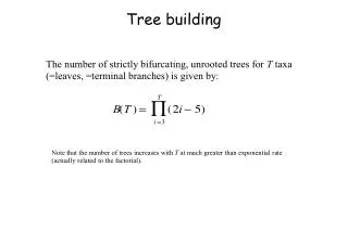
Tree building. The number of strictly bifurcating, unrooted trees for T taxa (=leaves, =terminal branches) is given by:. Note that the number of trees increases with T at much greater than exponential rate (actually related to the factorial). Tree building strategy. T3. T3. T3. T2. T2.

Tree building
E N D
Presentation Transcript
Tree building The number of strictly bifurcating, unrooted trees for T taxa (=leaves, =terminal branches) is given by: Note that the number of trees increases with T at much greater than exponential rate (actually related to the factorial).
Tree building strategy T3 T3 T3 T2 T2 T2 T6 T6 T6 T3 a b T2 c T6 T4 T4 f f b e a b e a d d d e c c f T4 Evaluate all trees, choose best, and repeat with another taxon.
Star decomposition A A B D D W B C E E C Now the hypothetical ancestor W is treated as a taxon (replacing D+E), and the process is repeated
Tree building methods • Exact: Construct trees and evaluate their scores according to a model such as: • Parsimony • Likelihood • Fitch-Margoliash distances. • This method gives all best trees, but is impractical for more than ca. 11 taxa. • Branch-and-bound strategy can make this practical for more taxa (ca. 20), and also gives all best trees. • Heuristic: Construct a tree from three of the taxa, add a fourth in all possible ways, evaluate tree scores, and choose the best tree(s) (or a group of good trees), then repeat additions until all taxa are added. • As in Exact, also choose model for tree evaluation. • Can get caught in local rather than global best “tree space.” • Should repeat tree construction with different (e.g. random) choice of starting tree. • Can further search for better trees by branch-swapping. • Star decomposition: Construct a star tree (all branches from the same point), then introduce internal branches by finding closest neighbors , repeating until the tree is fully resolved. • Neighbor-joining and clustering (e.g. UPGMA) methods. • Nodes are treated as taxa in subsequent iterations.
Methods to calculate distance on aligned nucleic acid sequences We assume a Markov general time reversible model, so most distance methods utilize some form of the following matrix: Where µ = mutation rate, a,b,c,d,e, and f are relative rate parameters for the various substitutions, and C G and T are frequency parameters for A, C, G, and T, respectively, in the sequences.
Jukes-CantorEqually weighting all changes and assuming equal frequencies of the bases
Kimura 2-parameter model:A matrix with a transition bias , and equal base frequencies:
Kimura 2-parameter:A more general model, taking into account base frequencies: But note that this assumes similar base frequencies in all the sequences (various approaches, such as Hadamard matrix techniques are used where base biases are different between taxa).
Maximum likelihood:Substitution matrix depends on evolutionary time The time (t) is estimated (in arbitrary units) by branch length, which in turn is estimated by Nelson approximation (beyond our consideration).
Tree building:Likelihood Conditional likelihoods for each branch are multiplied (L0*L1*L2*…) to get the likelihoods of character states at all inferred nodes. Since more than one tree may explain the character states, the likelihoods for all such trees are added. The products are typically very small, so they are converted to logarithms. The likelihood of the overall phylogeny is the product of the total likelihoods for the individual characters. This is calculated by adding the lnL for each character. The result is reported as the ln likelihood of the inferred tree (a negative number).
Refinements to distance and likelihood methods (better models) • Different sites mutate (fix mutations) at different rates. • Gamma distributions can be incorporated in the calculations • Different taxa may have different base frequencies. • Hadamard conjugation (description beyond this course) developed in part to address this. Hadamard conjugation is practical only for trees of very few taxa.
Parsimony vs. Distance vs. Likelihood • Parsimony • Intermediate speed (sometimes branch and bound can be very rapid) • Cladistic • View character changes on branches • Good for very similar sequences • Can be “positively misled” by long branches • Early diverged and/or rapidly evolved lineages will tend to group together. • Address (in part) by greater taxon sampling (always a good thing) • Distance • Fastest • Can use models that incorporate numerous real-life situations • Good for sequences of intermediate similarities • Signal can be lost on deeper branches • Likelihood • Basically a highly sophisticated parsimony • Most realistic of the models • Most robust to deviations from model • Least subject to long branch attraction • Very computationally intensive: the slowest of the methods
Outgroup rooting Cpurp20102 Echinodot201937 Eamar200743So Ebaco90167At Efest90661Frr Ebaco200745Cv Ebrom200749Be Eelym200850Evr Eglyc200747Gs Ebrac201561Bee Eclar200742Hl Etyph200740Dg Esylv200751Bs 010503 Nao 50 changes
Outgroup rooting Cpurp20102 Echinodot201937 Eamar200743So Ebaco90167At Efest90661Frr Ebaco200745Cv Ebrom200749Be Eelym200850Evr Eglyc200747Gs Ebrac201561Bee Eclar200742Hl Etyph200740Dg Esylv200751Bs 010503 Nao 50 changes
Outgroup rooting Cpurp20102 Echinodot201937 Eamar200743So Ebaco90167At Efest90661Frr Ebaco200745Cv Ebrom200749Be Eelym200850Evr Eglyc200747Gs Ebrac201561Bee Eclar200742Hl Etyph200740Dg Esylv200751Bs 010503 Nao 50 changes
Midpoint rooting 23 Eamar200743So 1 24 3 Ebaco90167At 31 15 Efest90661Frr 11 Ebaco200745Cv 4 44 Ebrom200749Be 9 21 5 Eelym200850Evr 31 Eglyc200747Gs 18 Ebrac201561Bee 18 14 Eclar200742Hl 15 13 28 Etyph200740Dg 10 Esylv200751Bs 18 010503 Nao 10 changes
Likelihood trees with lots of taxa Done in 2004, with dnaml in PHYLIP, on an Athelon 1.4 GHz PC running Linux: one iteration of random sequence addition. Time taken for each, about 8 hr. Run on PhyML at Phylogeny.fr, Jan 25, 2012: less than 6 minutes.
Bootstrap and Jackknife: Monte Carlo methods Original data Eam200743S TGGAGATCGTTTAATTA Eba76552A1 .......T......... Ebr2007521 C..........A..... Ebromi9608 ...............C. Eel2008505 .T........C...... Efestuc283 ................G Egl200747G .............C... Esy200748B .....GC.......... Esy200751B ...C.GC...C...... Ety200738A .....GC.......C.. Ety201666P ..A.TGC.......C.. Ety201667P .....G........... Ncoenop19T ............T.... Nineb818Ai ........CC....... Sample with replacement (bootstrap) Eam200743S ATAATTGGACGGATAGT Eba76552A1 .........T....... Ebr2007521 .C...........A... Ebromi9608 ................. Eel2008505 ......T.........C Efestuc283 G..G............. Egl200747G ........C........ Esy200748B ..G..C......G.... Esy200751B ..G..C......G.C.C Ety200738A ..G..C......G.... Ety201666P ..G..C.....AG..T. Ety201667P ..G.........G.... Ncoenop19T ................. Nineb818Ai ....C..C..C...... Original data Eam200743S TGGAGATCGTTTAATTA Eba76552A1 .......T......... Ebr2007521 C..........A..... Ebromi9608 ...............C. Eel2008505 .T........C...... Efestuc283 ................G Egl200747G .............C... Esy200748B .....GC.......... Esy200751B ...C.GC...C...... Ety200738A .....GC.......C.. Ety201666P ..A.TGC.......C.. Ety201667P .....G........... Ncoenop19T ............T.... Nineb818Ai ........CC....... Sample half without replacement (jackknife) Eam200743S AATTGGTAA Eba76552A1 ......... Ebr2007521 ..CA..... Ebromi9608 ......C.. Eel2008505 ......... Efestuc283 .G....... Egl200747G ........C Esy200748B .......G. Esy200751B C......G. Ety200738A .......G. Ety201666P ....T..G. Ety201667P .......G. Ncoenop19T ......... Nineb818Ai .....C...
Bootstrap and Jackknife: 1000 replicates of jackknife Eamar200743So 64 Ebaco90167At 100 Efest90661Frr Ebaco200745Cv 79 Ebrom200749Be 98 76 Eelym200850Evr Eglyc200747Gs Ebrac201561Bee 100 Eclar200742Hl 100 100 Etyph200740Dg Esylv200751Bs 010503 Nao
Comparing gene trees • Permutation homogeneity test • Kishino-Hasegawa test • Templeton signed rank test
Scoring matrices: e.g. PAM • The PAM1 matrix is estimated to represent likelihoods of changes in a 1 million years of divergence. • These values were calculated from comparisons of polypeptide sequences in databases. • To calculate the matrix for 2 million years, square the matrix as shown in the next slide. • To calculate the matrix for n million years, multiply the PAM1 matrix by itself n times. • Note that for PAM250 the likelihood for a residue to remain the same (F -> F in this example) is much lower than for PAM1, and likelihoods of change are much higher. • Same concept for BLOSUM matrices • BLOSUM scores were derived from local multiple alignments. • PAM scores were derived from global multiple alignments.
Calculating substitution scoring matrices aa1 aa2 aa3 --> ________________ aa1 | a b c aa2 | d e f aa3 | g h I … aa1 aa2 aa3 --> ________________ aa1 | a b c aa2 | d e f aa3 | g h I … aa1 aa2 aa3 --> ________________ aa1 | A B C aa2 | D E F aa3 | G H I … A = a2 + bd + cg +… B = ab + be + ch +… C = ac + bf + ci +… D = da + ed + fg +…, etc. … =
Scoring matrices:BLOSUM62 in half bits* *2ln2(score)
Gene/sequence relationships • Homologues (adj., homologous): derived from the same (“common”) ancestral gene • “homology”“similarity” • Orthologues (adj., orthologous): Related by descent from the common ancestor of the individuals possessing them • Paralogues (adj., paralogous): Derived from gene duplication; not orthologues • Analogues (adj., analogous): Related by convergent evolution; not homologues • Xenologues (adj. xenologous): From another species by horizontal transfer
Problems of homology • Paralogy • Chimeric genes • Xenology
Paralogy time A a B b C c time of divergence A-C a-c A-B a-b A-b a-B C-c
For orthologous genes, do the gene trees necessarily reflect species trees?