Download
1 / 58
580 likes | 737 Vues
Role of Stein’s Lemma in Guaranteed Training of Neural Networks. Anima Anandkumar. NVIDIA and Caltech. Non-Convex Optimization. ► Multiple local optima ► In high dimensions possibly exponential local optima. ► Unique optimum: global/local.

E N D
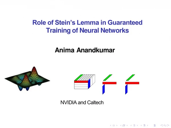
Role of Stein’s Lemma in Guaranteed Training of Neural Networks AnimaAnandkumar NVIDIA and Caltech
Non-Convex Optimization ► Multiple localoptima ► In high dimensions possibly exponential localoptima ► Unique optimum: global/local How to deal with the challenge ofnon-convexity? Finding the globaloptimum 3/33
Local Optima inNeuralNetworks Example of Failure ofBackpropagation y y=−1 y=1 σ(·) σ(·) Localoptimum Globaloptimum x1 x2 x Exponential (in dimensions) no. of local optima forbackpropagation
Guaranteed Learning throughTensor Methods Replace the objectivefunction Cross Entropy vs. Best Tensordecomp. Preserves Global Optimum (infinitesamples) T (x): empirical tensor, T (θ): low rank tensorbased on θ. 2 argminIT(x)−T(θ) I F θ Dataset1 Dataset2 Finding globally opt tensordecomposition Model Class Simple algorithms succeed under mild andnatural conditions for many learningproblems.
Guaranteed Training of Neural Networks using Tensor Decomposition Majid Janzamin Hanie Sedghi
Method of Momentsfor a NeuralNetwork ► Supervised setting: observing {(xi,yi)} ► Non-linear transformations via activating functionσ(·) ► Random x andy: Momentpossibilities: E[y ⊗y], E[y⊗x], ... y σ(·)σ(·) E[y⊗x]=E[σ(ATx)⊗x] 1 ⇒ A1 No linear transformation of A1.× x2 x3 xx1 One solution: Linearization by using Stein’s Lemma Derivative −−−−−−→ σ'(·)A1T σ(ATx) 1 26/33
Moments of a NeuralNetwork y E[y|x]:=f(x)=(a2,σ(AT1x)) a2 σ(·)σ(·) A= 1 x1 x2 x3 x “Score Function Features for Discriminative Learning: Matrix and Tensor Framework” byM. Janzamin, H. Sedghi, and A. , Dec.2014.
Moments of a NeuralNetwork y E[y|x]:=f(x)=(a2,σ(AT1x)) Moments using score functionsS(·) a2 σ(·) σ(·) A= 1 x1 x2 x3 x “Score Function Features for Discriminative Learning: Matrix and Tensor Framework” byM. Janzamin, H. Sedghi, and A. , Dec.2014.
Moments of a NeuralNetwork y E[y|x]:=f(x)=(a2,σ(AT1x)) Moments using score functionsS(·) E [y ·S1(x)]= + a2 σ(·) σ(·) A= 1 x x x x 1 2 3 “Score Function Features for Discriminative Learning: Matrix and Tensor Framework” byM. Janzamin, H. Sedghi, and A. , Dec.2014.
Moments of a NeuralNetwork y E[y|x]:=f(x)=(a2,σ(AT1x)) Moments using score functionsS(·) E [y ·S2(x)]= + a2 σ(·) σ(·) A= 1 x1 x2 x3 x “Score Function Features for Discriminative Learning: Matrix and Tensor Framework” byM. Janzamin, H. Sedghi, and A. , Dec.2014.
Moments of a NeuralNetwork y E[y|x]:=f(x)=(a2,σ(AT1x)) Moments using score functionsS(·) E [y ·S3(x)]= + a2 σ(·) σ(·) A= 1 x1 x2 x3 x “Score Function Features for Discriminative Learning: Matrix and Tensor Framework” byM. Janzamin, H. Sedghi, and A. , Dec.2014.
Moments of a NeuralNetwork y E[y|x]:=f(x)=(a2,σ(AT1x)) Moments using score functionsS(·) E [y ·S3(x)]= + a2 σ(·) σ(·) A= 1 x1 x2 x3 x ► Linearization using derivativeoperator. Stein’s lemma φm(x) : m-th order derivativeoperator “Score Function Features for Discriminative Learning: Matrix and Tensor Framework” byM. Janzamin, H. Sedghi, and A. , Dec.2014.
Moments of a NeuralNetwork y E[y|x]:=f(x)=(a2,σ(AT1x)) Moments using score functionsS(·) E [y ·S3(x)]= + a2 σ(·) σ(·) A= 1 x1 x2 x3 x Theorem (Score function property) When p(x) vanishes atboundary, Sm(x) exists, and m-differentiable function f(·) Stein’s lemma (m) E[y·S (x)]=E[f(x)·S (x)]=E [∇ f (x)]. . m m x “Score Function Features for Discriminative Learning: Matrix and Tensor Framework” byM. Janzamin, H. Sedghi, and A. , Dec.2014.
Stein’s Lemma through Score functions ► Continuous x with pdfp(·): S1(x):=−∇xlogp(x) Input: S1(x) ∈Rd x ∈Rd 28/33
Stein’s Lemma through Score functions ► Continuous x with pdfp(·): ► mth-order scorefunction: Input: S1(x) ∈Rd x ∈Rd m∇(m)p(x) Sm(x) :=(−1) p(x) 28/33
Stein’s Lemma through Score functions ► Continuous x with pdfp(·): ► mth-order scorefunction: x ∈Rd m∇(m)p(x) Sm(x) :=(−1) Input: S2(x) ∈Rd×d p(x) 28/33
Stein’s Lemma through Score functions ► Continuous x with pdfp(·): ► mth-order scorefunction: x ∈Rd m∇(m)p(x) Sm(x) :=(−1) Input: S3(x) ∈Rd×d×d p(x) 28/33
Stein’s Lemma through Score functions ► Continuous x with pdfp(·): ► mth-order scorefunction: x ∈Rd m∇(m)p(x) Sm(x) :=(−1) Input: S3(x) ∈Rd×d×d p(x) ► For Gaussian x ∼ N(0, I): orthogonal Hermite polynomials S1(x)=x, S2(x)=xxT−I, . .. 28/33
Stein’s Lemma through Score functions ► Continuous x with pdfp(·): ► mth-order scorefunction: x ∈Rd m∇(m)p(x) Sm(x) :=(−1) Input: S3(x) ∈Rd×d×d p(x) ► For Gaussian x ∼ N(0, I): orthogonal Hermite polynomials S1(x)=x, S2(x)=xxT−I, . .. Application of Stein’s Lemma ► Providing derivative information: let E[y|x] := f (x),then ► For Gaussian x ∼ N(0, I): orthogonal Hermite polynomials S1(x)=x, S2(x)=xxT−I, . .. 28/33
Training Neural Networks withTensors Realizable: E[y · Sm(x)] has CP tensordecomposition. M. Janzamin, H. Sedghi, and A., “Beating the Perils of Non-Convexity: Guaranteed Trainingof Neural Networks using Tensor Methods,” June.2015. A. Barron, “Approximation and Estimation Bounds for Artificial Neural Networks,” Machine Learning,1994.
Training Neural Networks withTensors Realizable: E[y · Sm(x)] has tensordecomposition. Non-realizable: Theorem (training neuralnetworks) ˆ ˜ 2 2 f E[|f(x)−f(x) | ] ≤ O(C /k)+O(1/n). For small enough C x f n samples, k number ofneurons M. Janzamin, H. Sedghi, and A., “Beating the Perils of Non-Convexity: Guaranteed Trainingof Neural Networks using Tensor Methods,” June.2015. A. Barron, “Approximation and Estimation Bounds for Artificial Neural Networks,” Machine Learning,1994.
Training Neural Networks withTensors First guaranteed method for training neuralnetworks M. Janzamin, H. Sedghi, and A., “Beating the Perils of Non-Convexity: Guaranteed Trainingof Neural Networks using Tensor Methods,” June.2015. A. Barron, “Approximation and Estimation Bounds for Artificial Neural Networks,” Machine Learning,1994.
Background on optimization landscape of tensor decomposition
Notion of TensorContraction Extends the notion of matrixproduct Matrixproduct TensorContraction
Symmetric TensorDecomposition = + +··· T=v1⊗3 +v2⊗3 +···, A.,R.Ge,D.Hsu,S.Kakade,M.Telgarsky,“TensorDecompositionsforLearningLatent Variable Models,” JMLR2014.
Symmetric TensorDecomposition Tensor PowerMethod = + +··· T(v,v,·) v →IT(v,v,·)I. 2 2 T(v,v,·)=(v,v1)v1+(v,v2)v2 A.,R.Ge,D.Hsu,S.Kakade,M.Telgarsky,“TensorDecompositionsforLearningLatent Variable Models,” JMLR2014.
Symmetric TensorDecomposition Tensor PowerMethod = + +··· T(v,v,·) v→IT(v,v,·)I . 2 2 T(v,v,·)=(v,v1)v1+(v,v2)v2 OrthogonalTensors v1 ⊥v2. T(v1,v1,·)=λ1v1. A.,R.Ge,D.Hsu,S.Kakade,M.Telgarsky,“TensorDecompositionsforLearningLatent Variable Models,” JMLR2014.
Symmetric TensorDecomposition Tensor PowerMethod = + +··· T(v,v,·) v→IT(v,v,·)I . 2 2 T(v,v,·)=(v,v1)v1+(v,v2)v2 OrthogonalTensors = v1 ⊥v2. T(v1,v1,·)=λ1v1. A.,R.Ge,D.Hsu,S.Kakade,M.Telgarsky,“TensorDecompositionsforLearningLatent Variable Models,” JMLR2014.
Symmetric TensorDecomposition Tensor PowerMethod = + +··· T(v,v,·) v→IT(v,v,·)I. T(v,v,·)=(v,v1)2v1+(v,v2)2v2 Exponential no. of stationary points for powermethod: T(v,v,·)=λv A.,R.Ge,D.Hsu,S.Kakade,M.Telgarsky,“TensorDecompositionsforLearningLatent Variable Models,” JMLR2014.
Symmetric TensorDecomposition Tensor PowerMethod = + +··· T(v,v,·) v→IT(v,v,·)I. T(v,v,·)=(v,v1)2v1+(v,v2)2v2 Exponential no. of stationary points for powermethod: T(v,v,·)=λv Stable Unstable Other statitionarypoints A.,R.Ge,D.Hsu,S.Kakade,M.Telgarsky,“TensorDecompositionsforLearningLatent Variable Models,” JMLR2014.
Symmetric TensorDecomposition Tensor PowerMethod = + +··· T(v,v,·) v→IT(v,v,·)I. T(v,v,·)=(v,v1)2v1+(v,v2)2v2 Exponential no. of stationary points for powermethod: T(v,v,·)=λv For power method on orthogonal tensor, no spurious stablepoints A.,R.Ge,D.Hsu,S.Kakade,M.Telgarsky,“TensorDecompositionsforLearningLatent Variable Models,” JMLR2014.
Non-orthogonal TensorDecomposition = + +··· T=v1⊗3 +v2⊗3 +···, A.,R.Ge,D.Hsu,S.Kakade,M.Telgarsky,“TensorDecompositionsforLearningLatent Variable Models,” JMLR2014.
Non-orthogonal TensorDecomposition Orthogonalization Input tensorT A.,R.Ge,D.Hsu,S.Kakade,M.Telgarsky,“TensorDecompositionsforLearningLatent Variable Models,” JMLR2014.
Non-orthogonal TensorDecomposition Orthogonalization T(W,W,W)=T˜ A.,R.Ge,D.Hsu,S.Kakade,M.Telgarsky,“TensorDecompositionsforLearningLatent Variable Models,” JMLR2014.
Non-orthogonal TensorDecomposition Orthogonalization v1v2 W v˜1v˜2 T(W,W,W)=T˜ A.,R.Ge,D.Hsu,S.Kakade,M.Telgarsky,“TensorDecompositionsforLearningLatent Variable Models,” JMLR2014.
Non-orthogonal TensorDecomposition Orthogonalization v1v2 W v˜1v˜2 T(W,W,W)=T˜ T˜=T(W,W,W)=v˜1⊗3+v˜2⊗3+···, = + A.,R.Ge,D.Hsu,S.Kakade,M.Telgarsky,“TensorDecompositionsforLearningLatent Variable Models,” JMLR2014.
Non-orthogonal TensorDecomposition Orthogonalization v1v2 W v˜1v˜2 T(W,W,W)=T˜ Find W using SVD of MatrixSlice + M=T(·,·,θ)= A.,R.Ge,D.Hsu,S.Kakade,M.Telgarsky,“TensorDecompositionsforLearningLatent Variable Models,” JMLR2014.
Non-orthogonal TensorDecomposition Orthogonalization v1v2 W v˜1v˜2 T(W,W,W)=T˜ Orthogonalization: invertible when vi’s linearlyindependent. A.,R.Ge,D.Hsu,S.Kakade,M.Telgarsky,“TensorDecompositionsforLearningLatent Variable Models,” JMLR2014.
Non-orthogonal TensorDecomposition Orthogonalization v1v2 W v˜1v˜2 T(W,W,W)=T˜ Orthogonalization: invertible when vi’s linearly independent. Recovery of Network Weights under LinearIndependence A.,R.Ge,D.Hsu,S.Kakade,M.Telgarsky,“TensorDecompositionsforLearningLatent Variable Models,” JMLR2014.
Perturbation Analysis for TensorDecomposition Well understood for matrix decomposition vs. hard for polynomials. Contribution: first results for tensordecomposition. A.,R.Ge,D.Hsu,S.Kakade,M.Telgarsky,“TensorDecompositionsforLearningLatent Variable Models,” JMLR2014.