Maps and hashing
Maps and hashing. Maps. A map models a searchable collection of key-value entries Typically a key is a string with an associated value (e.g. salary info) The main operations of a map are for searching, inserting, and deleting items Multiple entries with the same key are not allowed

Maps and hashing
E N D
Presentation Transcript
Maps and hashing Hashing
Maps • A map models a searchable collection of key-value entries • Typically a key is a string with an associated value (e.g. salary info) • The main operations of a map are for searching, inserting, and deleting items • Multiple entries with the same key are not allowed • Applications: • address book • student-record database • Salary information,etc Hashing
The Map ADT • Map ADT methods: • Get(k): if the map M has an entry with key k, return its associated value; else, return null • Put (k, v): insert entry (k, v) into the map M; if key k is not already in M, then return null; else, return old value associated with k • Remove (k): if the map M has an entry with key k, remove it from M and return its associated value; else, return null • Size(), isEmpty() • Keys(): return an iterator of the keys in M • Values(): return an iterator of the values in M Hashing
Example Operation Output Map isEmpty() true Ø put(5,A) null (5,A) It returns null because it is not in M put(7,B) null (5,A),(7,B) put(2,C) null (5,A),(7,B),(2,C) put(8,D) null (5,A),(7,B),(2,C),(8,D) put(2,E) C(5,A),(7,B),(2,E),(8,D) get(7) B(5,A),(7,B),(2,E),(8,D) get(4) null (5,A),(7,B),(2,E),(8,D) Because 4 is not in M get(2) E (5,A),(7,B),(2,E),(8,D) size() 4 (5,A),(7,B),(2,E),(8,D) remove(5) A (7,B),(2,E),(8,D) Remove 5 and return A remove(2) E (7,B),(8,D) get (2) null (7,B),(8,D) Because 4 is not in M isEmpty() false (7,B),(8,D) Because there are 2 in M Hashing
Comparison to java.util.Map Map ADT Methods java.util.Map Methods size() size() isEmpty() isEmpty() get(k) get(k) put(k,v) put(k,v) remove(k) remove(k) All same except: keys() keySet().iterator() values() values().iterator() Hashing
Performance: put takes O(1) time, since we can insert the new item at the beginning or at the end of the sequence get and remove take O(n) time since in the worst case (the item is not found) we traverse the entire sequence to look for an item with the given key The unsorted list implementation is effective only for maps of small size or for maps in which puts are the most common operations, while searches and removals are rarely performed (e.g., historical record of logins to a workstation) Performance of a List-Based Map Hashing
Hashing Hashing
Content • Idea: when using various operations on binary search trees, we use hash table ADT • Hashing: implementation of hash tables for insert and find operations is called hashing. • Collision: when two keys hash to the same value • Resolving techniques for collision using linked lists • Rehashing: when a hash table is full, then operations will take longer time. Then we need to build a new double sized hash table. (HWLA??? Why double sized..) • Extendible hashing: for fitting large data in main memory Hashing
Hashing as a Data Structure • Performs operations in O(1) • Insert • Delete • Find • Is not suitable for • FindMin • FindMax • Sort or output as sorted Hashing
General Idea • Array of Fixed Size (TableSize) • Search is performed on some part of the item (Key) • Each key is mapped into some number between 0 and (TableSize-1) • Mapping is called a hash function • Ensure that two distinct keys get different cells • Problem: Since there are a finite # of cells and virtually inexhaustible supply of keys, we need a hash function to distribute the keys evenly among the cells!!!!!! Hashing
A hash functionh maps keys of a given type to integers in a fixed interval [0, N- 1] Example:h(x) =x mod Nis a hash function for integer keys The integer h(x) is called the hash value of key x A hash table for a given key type consists of Hash function h Array (called table) of size N When implementing a map with a hash table, the goal is to store item (k, o) at index i=h(k) Hash Functions and Hash Tables Hashing
0 1 025-612-0001 2 981-101-0002 3 4 451-229-0004 … 9997 9998 200-751-9998 9999 Example • We design a hash table for a map storing entries as (SSN, Name), where SSN (social security number) is a nine-digit positive integer • Our hash table uses an array of sizeN= 10,000 and the hash functionh(x) = last four digits of x Hashing
Hash Functions • Easy to compute • Key is of type Integer • reasonable strategy is to return Key ModTableSize-1 • Key is of type String (mostly used in practice) • Hash function needs to be chased carefully! Eg. Adding up the ASCII values of the characters in the string Proper selection of hash function is required Hashing
Hash Function (Integer) • Simply return Key % TableSize • Choose carefully TableSize • TableSize is 10, all keys end in zero??? • To avoid such pitfalls, choose TableSize a prime number Hashing
Hash Function I (String) • Adds up ASCII values of characters in the string • Advantage: Simple to implement and computes quickly • Disadvantage: If TableSize is large (see Fig.5.2 in your book), function does not distribute keys well • Example: Keys are at most 8 characters. Maximum sum (8*256 = 2048), but TableSize 10007. Only 25 percent could be filled. Hashing
Hash Function II (String) • Assumption: Key has at least 3 characters • Hash Function: (26 characters for alphabet + blank) key[0] + 27 * key[1] + 272 * key[2] • Advantage: Distributes better than Hash Function I, and easy to compute. • Disadvantage: • 263 = 17,576 possible combinations of 3 characters • However, English has only 2,851 different combinations by a dictionary check. • HWLA: Explain why? Read p.157 for the answer. • Similar to Hash Function 1, it is not appropriate, if the hash table is reasonably large! Hashing
Hash Function III (String) • Idea: Computes a polynomial function of Key’s characters P(Key with n+1 characters) = Key[0]+37Key[1]+372Key[2]+...+37nKey[n] • If find 37n then sum up complexity O(n2) • Using Horner’s rule complexity drops to O(n) ((Key[n]*37+Key[n-1])*37+...+Key[1])*37+Key[0] • Very simple and reasonably fast method, but there will be complexity problem if the key-characters are very long! • The lore is to avoid using all characters to set a key. Eg: the keys could be a complete street address. The hash function might include a couple of characters from the street address, and may be a couple of characters from the city name, or zipcode. • Think of other options??? Quiz: Lately 31 is proposed instead of 37.. Why not 19? Hashing
Hash Function III (String) public static int hash( String key, int tableSize ) { int hashVal = 0; for( int i = 0; i < key.length( ); i++ ) hashVal = 37 * hashVal + key.charAt( i ); hashVal %= tableSize; if( hashVal < 0 ) hashVal += tableSize; return hashVal; } Hashing
Collisions occur when different elements are mapped to the same cell 0 1 025-612-0001 2 3 4 451-229-0004 981-101-0004 Collision Hashing
Collision • When an element is inserted, it hashes to the same value as an already inserted element we have collision. (e.g. 564 and 824 will collide at 4) • Example: Hash Function (Key % 10) Hashing
Solving Collision • Separate Chaining: • keep a list of all elements hashing to the same value, and traverse the list to find corresponding hash. Hint: lists should be large and kept as prime number table size to ensure a good distribution. (Limited use due to space limitations of lists, and needs linked lists!!!) • Open Addressing: • at a collision, search for alternative cells until finding an empty cell. • Linear Probing • Quadratic Probing • Double Hashing Hashing
Solving Collision • Define: The load factor: Lamda= #of elements/Tablesize • HWLA: Search Internet for other techniques (is there any algorithm without using a linked list) • A) Binary search tree • B) Using another hash table • Explain why we donot use A and B? • Solution: If the table size is large and a proper hash function is used, then the list should be short. Therefore, it is not worth to find anything more complicated!!! Hashing
Separate Hashing Insert keys [ 9, 8, 7, 6, 5,4,3,2,1,0] into the hast table using h(x)= x2 % TableSize • Separate Chaining: let each cell in the table point to a linked list of entries that map there • Keep a list of all elements that hash to the same value • Each element of the hash table is a Link List • Separate chaining is simple, but requires additional memory outside the table Hashing
Load Factor (Lambda): • Lambda: the number of elements in hash table divided by the Tablesize. (Eg. Lambda = 1 for the table.) • To perform a search is the constant time required evaluate the hash function + the time to traverse the list • Unsuccessful search: (Lambda) nodes to be examined, on average. • Successful search: (1+Lambda/2) links to be traversed. • Note: Average number of other nodes in Tablesize of N with M lists: • (N-1)/M=N/M-1/M= Lambda-1/M=Lambda for large M. • i.e., Tablesize is not important, but load factor is.. • So, in separate chaining, Lambda should be kept nearer to 1. • i.e. Make the has table as large as the number of elements expected (for possible collision). • Remember also that the tablesize should be prime for ensuring a good distribution….... Hashing
Separate Hashing /** * Construct the hash table. */ public SeparateChainingHashTable( ){ this( DEFAULT_TABLE_SIZE ); } /** * Construct the hash table. * @param size approximate table size. */ public SeparateChainingHashTable( int size ){ theLists = new LinkedList[ nextPrime( size ) ]; for( int i = 0; i < theLists.length; i++ ) theLists[ i ] = new LinkedList( ); } Hashing
Separate Hashing • Find • Use hash function to determine which list to traverse • Traverse the list to find the element public Hashable find( Hashable x ){ return (Hashable)theLists[ x.hash( theLists.length ) ].find(x).retrieve( ); } Hashing
Separate Hashing • Insert • Use hash function to determine in which list to insert • Insert element in the header of the list public void insert( Hashable x ){ LinkedList whichList = theLists[x.hash(theLists.length) ]; LinkedListItr itr = whichList.find( x ); if( itr.isPastEnd( ) ) whichList.insert( x, whichList.zeroth( ) ); } Hashing
Separate Hashing • Delete • Use hash function to determine from which list to delete • Search element in the list and delete public void remove( Hashable x ){ theLists[ x.hash( theLists.length ) ].remove( x ); } Hashing
Separate Hashing • Advantages • Solves the collision problem totally • Elements can be inserted anywhere • Disadvantages • Need the use of link lists.. And, all lists must be short to get O(1) time complexity otherwise it take too long time to compute… Hashing
Separate Hashing needs extra space!!! • Alternatives to Using Link Lists • Binary Trees • Hash Tables However, If the Tablesize is large and a good hash function is used, all the lists expected to be short already, i.e., no need to complicate!!! Instead of the above alternative techniques, we use Open Addressing>>>>> Hashing
Open Addressing • Solving collisions without using any other data structure such as link list • this is a major problem especially for other languages!!! • Idea: If collision occurs, alternative cells are tried until an empty cell is found =>>> Cells h0(x), h1(x), ..., are tried in succession • hi(x)=(hash(x) + f(i)) % TableSize • The function f is the collision resolution strategy with f(0)=0. • Since all data go inside the table, Open addressing technique requires the use of bigger table as compared to separate chaining. • Lambda should be less than 0.5. (it was 1 for separate hashing) Hashing
Open Addressing • Depending on the collision resolution strategy, f, we have • Linear Probing: f(i) = i • Quadratic Probing: f(i) = i2 • Double Hashing: f(i) = i hash2(x) Hashing
Linear Probing f(i) = i is the amount to trying cells sequentially in search of an empty cell. • Advantages: Easy to compute • Disadvantages: • Table must be big enough to get a free cell • Time to get a free cell may be quite large • Primary Clustering • Any key that hashes into the cluster will require several attempts to resolve the collision Hashing
Open addressing: the colliding item is placed in a different cell of the table Linear probing handles collisions by placing the colliding item in the next (circularly) available table cell Each table cell inspected is referred to as a “probe” Colliding items lump together, causing future collisions to cause a longer sequence of probes Example: h(x) = x mod13 Insert keys 18, 41, 22, 44, 59, 32, 31, 73, in this order Example: Linear Probing 0 1 2 3 4 5 6 7 8 9 10 11 12 41 18 44 59 32 22 31 73 0 1 2 3 4 5 6 7 8 9 10 11 12 Hashing
Example in the book: Linear Probing Insert keys [ 89, 18, 49, 58, 69] into a hast table using hi(x)=(hash(x) + i) % TableSize Hashing
First collision occurs when 49 is inserted. (then, put in the next available cell, i.e. cell 0) • 58 collides with 18, 89, and then 49 before an empty cell is found three away • The collision 69 is handled as above. • Note: insertions and unsuccessful searches require the same number of probes. • Primary clustering? If table is big enough, a free cell will always be found (even if it takes long time!!!) If the table is relatively empty (lowerLambda) , yet key may require several attempts to resolve collision. Then, blocks of occupied cells start forming, i.e., need to add to cluster ….. Hashing
Quadratic Probing • Eliminates Primary Clustering problem • Theorem: If quadratic probing is used, and the table size is prime, then a new element can always be inserted if the table is at least half empty • Secondary Clustering • Elements that hash to the same position will probe the same alternative cells Hashing
Quadratic Probing Insert keys [ 89, 18, 49, 58, 69] into a hast table using hi(x)=(hash(x) + i2) % TableSize Hashing
Quadratic Probing /** * Construct the hash table. */ public QuadraticProbingHashTable( ) { this( DEFAULT_TABLE_SIZE ); } /** * Construct the hash table. * @param size the approximate initial size. */ public QuadraticProbingHashTable( int size ) { allocateArray( size ); makeEmpty( ); } Hashing
Quadratic Probing /** * Method that performs quadratic probing resolution. * @param x the item to search for. * @return the position where the search terminates. */ private int findPos( Hashable x ) { /* 1*/ int collisionNum = 0; /* 2*/ int currentPos = x.hash( array.length ); /* 3*/ while( array[ currentPos ] != null && !array[ currentPos ].element.equals( x ) ) { /* 4*/ currentPos += 2 * ++collisionNum - 1; /* 5*/ if( currentPos >= array.length ) /* 6*/ currentPos -= array.length; } /* 7*/ return currentPos; } Hashing
Double hashing uses a secondary hash function d(k) and handles collisions by placing an item in the first available cell of the series (i+jd(k)) mod Nfor j= 0, 1, … , N - 1 The secondary hash function d(k) cannot have zero values The table size N must be a prime to allow probing of all the cells Common choice of compression function for the secondary hash function: d2(k) =q-k mod q where q<N q is a prime The possible values for d2(k) are1, 2, … , q Double Hashing Hashing
Double Hashing • Popular choice: f(i)=i. hash2(x) i.e., apply a second hash function to x and probe at a distance hash2(x) , 2hash2(x) , 3 hash2(x) … • hash2(x) = R – (x % R) • Poor choice of hash2(x) could be disastrous Observe: hash2(x) =xmod9 would not work if 99 were inserted into the input in the previous example • R should also be a prime number smaller than TableSize • If double hashing is correctly implemented, simulations imply that the expected number of probes is almost the same as for a random collision resolution strategy Hashing
Example of Double Hashing • Consider a hash table storing integer keys that handles collision with double hashing • N= 13 • h(k) = k mod13 • d(k) =7 - k mod7 • Insert keys 18, 41, 22, 44, 59, 32, 31, 73, in this order 0 1 2 3 4 5 6 7 8 9 10 11 12 31 41 18 32 59 73 22 44 0 1 2 3 4 5 6 7 8 9 10 11 12 Hashing
Example in the book Double Hashing Hi(x) = (x + i (R – (x mod R))) % N, R = 7, N=10 The first collision occurs when 49 is inserted hash2 (49)=7-0=7 thus, 49 is inserted in position 6.hash2(58)=7-2=5, so 58 is inserted at location 3. Finally, 69 collides and is inserted at a distance hash2(69)=7-6=1 away. Observe a bad scenario: if we had an input 60, then what happens? First, 60 collides with 69 in the position 0. Since hash2 (60)=7-4=3, we would then try positions 3, 6, 9, and then 2 until an empty cell is found. Hashing
Rehashing • If Hash Table gets too full, running time for the operations will start taking too long time • Insertions might fail for open addressing with quadratic probing • Solution: Rehashing build another table that is about twice as big…. • Rehashing is used especially when too many removals intermixed with insertions Hashing
Rehashing • Build another table that is about twice as big E.g. if N=11, then N’=23 • Associate a new hash function • Scan down the entire original hash table • Compute the new hash value for each nondeleted element. • Insert it in the new table Hashing
Rehashing • Very expensive operation; O(N) • Good news is that rehashing occurs very infrequently • If data structure is part of the program, effect is not noticeable. • If hashing is performed as part of an interactive system, then the unfortunate user whose insertion caused a rehash could observe a slowdown Hashing
Rehashing • When to apply rehashing? • Strategy1: As soon as the table is half full • Strategy2: Only when an insertion fails • Strategy3: When the table reaches a certain load factor • No certain rule for the best strategy! Since load factor is directly related to the performance of the system, 3rd strategy may work better.. Then what is the threshold??? Hashing
Example: Rehashing • Suppose 13,15,23, 24, and 6 are inserted into a hash table of size 7. • Assume h(x)= x mod 7, using linear probing we get the table on the left. • But table is 5/7 full, rehashing is required…. The new tablesize is 17. • 17 is the first prime number greater than 2*7 • The new h(x)=x mod17. Scanned the old table, insert the elements 6,13,15,23,24 (as shown in table on the right). Hashing
Rehashing private void allocateArray( int arraySize ) { array = new HashEntry[ arraySize ]; } private void rehash( ) { HashEntry [ ] oldArray = array; // Create a new double-sized, empty table allocateArray( nextPrime( 2 * oldArray.length ) ); currentSize = 0; // Copy table over for( int i = 0; i < oldArray.length; i++ ) if( oldArray[ i ] != null && oldArray[ i ].isActive) insert( oldArray[ i ].element ); return; } Hashing