Analysis of Climate Patterns: Impacts & Predictions
180 likes | 271 Vues
Explore the relationship between key climate variables and phenomena through regression analysis. Understand how volcanic aerosols, ENSO indices, sunspots, and more influence sea level pressure and surface temperature.

Analysis of Climate Patterns: Impacts & Predictions
E N D
Presentation Transcript
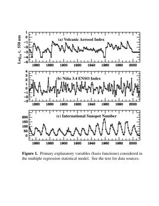
(a) Volcanic Aerosol Index Log10, 550 nm (b) Niña 3.4 ENSO Index (c) International Sunspot Number Figure 1. Primary explanatory variables (basis functions) considered in the multiple regression statistical model. See the text for data sources.
(a) Climatological Mean Sea Level Pressure, DJF (1979-2009) hPa (b) Climatological Sea Surface Temperature, DJF (1979-2009) oC Figure 2. Mean sea level pressure (a) and sea surface temperature (b) for the northern winter season (DJF), based on Hadley Centre data over the 1979 to 2009 period.
(a) Hadley Centre DJF SLP Change per -1 unit N3.4, 1880-2009 hPa hPa (b) Hadley Centre DJF SST Change per -1 unit N3.4, 1880-2009 oC oC Figure 3. Mean sea level pressure (a) and sea surface temperature (b) responses to a moderate La Niña event as estimated from a multiple regression analysis of 130 years of Hadley Centre data. Heavy dark lines enclose regions where the regression coefficients are significant at the 2 level.
(a) Hadley DJF SLP Change per +1 Unit of AO Index (1950-2009) hPa hPa hPa (b) Hadley DJF SST Change per +1 Unit of AO Index (1950-2009) oC oC OC Figure 4. Same format as Figure 3 but for the responses to a positive change in the Arctic Oscillation (AO) index, as estimated from a multiple regression analysis of 60 years of Hadley Centre data.
(a) Hadley DJF SLP Change per +130 Units of SSN (1880-2009) hPa hPa hPa (b) Hadley DJF SST Change per +130 Units of SSN (1880-2009) oC oC OC Figure 5. Same format as Figures 3 and 4 but for the SLP and SST responses to a positive change in the sunspot number of 130, as estimated from a multiple regression analysis of 130 years of Hadley Centre data.
(a) DJF SLP Change per 130 Units of SSN, Lag = 2 Years (b) DJF SLP Change per 130 Units of SSN, Lag = 1 Year (c) DJF SLP Change per 130 Units of SSN, Lag = +1 Year (d) DJF SLP Change per 130 Units of SSN, Lag = +2 Years hPa oC Figure 6. Dependence on phase lag of the Hadley Centre sea level pressure response to a change in SSN of +130. Same format as Figure 5a but for times of: (a) two years before solar maximum; (b) one year before solar maximum; (c) one year after solar maximum; and (d) two years after solar maximum.
(a) DJF SST Change per 130 Units of SSN, Lag = 2 Years (b) DJF SST Change per 130 Units of SSN, Lag = 1 Year (c) DJF SST Change per 130 Units of SSN, Lag = +1 Year (d) DJF SST Change per 130 Units of SSN, Lag = +2 Years hPa oC Figure 7. Dependence on phase lag of the Hadley Centre sea surface temperature response to a change in SSN of +130. Same format as Figure 6.
(a) O3 Change from 2D Model (Haigh 1994) (b) O3 Change from Observations (Soukharev & Hood 2006) (c) O3 Change from Observations + 2D Model Figure 8. Annual mean ozone percent change from solar minimum to maximum specified in each of the three EGMAM simulations as a function of latitude and pressure level (hPa). See the text.
(a) EGMAM DJF SLP Change per -1 unit N3.4, 2138-2665 hPa hPa hPa (b) EGMAM DJF SST Change per -1 unit N3.4, 2138-2665 oC oC Figure 9. Northern winter mean sea level pressure (a) and sea surface temperature (b) responses to a moderate La Niña event as estimated from a multiple regression analysis of the three EGMAM simulations, combined in series (176 3 years).
Figure 10. Scatter plot of monthly mean solar 10.7 cm radio flux (in solar flux units) versus monthly mean sunspot number over the 1948 to 2010 period. See the text.
(a) Simulation 1 DJF SLP Change per 130 Units F10.7 (2138-2313) hPa (b) Simulation 1 DJF SST Change per 130 Units F10.7 (2138-2313) oC Figure 11. Northern winter mean sea level pressure (a) and sea surface temperature (b) responses to a change of +130 units of the 10.7 cm radio flux (F10.7). The responses are estimated from a multiple regression analysis of EGMAM Simulation 1 (176 years), which assumed a solar cycle ozone variation based on a 2D model calculation (Figure 9a).
(a) Simulation 2 DJF SLP Change per 130 Units F10.7 (2138-2313) hPa hPa hPa (b) Simulation 2 DJF SST Change per 130 Units F10.7 (2138-2313) oC Figure 12. Same format as Figure 11 but based on a multiple regression analysis of EGMAM Simulation 2 (176 years), which assumed a solar cycle ozone variation based on observations (Figure 9b).
(a) Simulation 3 DJF SLP Change per 130 Units F10.7 (2138-2313) hPa (b) Simulation 3 DJF SST Change per 130 Units F10.7 (2138-2313) oC Figure 13. Same format as Figures 11 and 12 but based on a multiple regression analysis of EGMAM Simulation 3 (176 years), which assumed a solar cycle ozone variation based on observations at latitudes < 60o and on 2D model calculations at higher latitudes (Figure 9c).
(a) Simulation 1 DJF SLP Change per 130 Units F10.7 (2196-2300) hPa (b) Simulation 1 DJF SST Change per 130 Units F10.7 (2196-2300) oC Figure 14. Same format as Figure 11 but for a selected centennial period of Simulation 1 (105 years).
(a) Simulation 2 DJF SLP Change per 130 Units F10.7 (2152-2256) hPa (b) Simulation 2 DJF SST Change per 130 Units F10.7 (2152-2256) oC Figure 15. Same format as Figure 12 but for a selected centennial period of Simulation 2 (105 years).
(a) Simulation 3 DJF SLP Change per 130 Units F10.7 (2196-2300) hPa (b) Simulation 3 DJF SST Change per 130 Units F10.7 (2196-2300) oC Figure 16. Same format as Figure 13 but for a selected centennial period of Simulation 3 (105 years).
(a) S2 (2152-2256) DJF SLP Change / 130 F10.7, Lag = 2 Yr (b) S2 (2152-2256) DJF SLP Change / 130 F10.7, Lag = 1 Yr (c) S2 (2152-2256) DJF SLP Change / 130 F10.7, Lag = +1 Yr (d) S2 (2152-2256) DJF SLP Change / 130 F10.7, Lag = +2 Yr hPa Figure 17. Dependence on phase lag of the northern winter SLP response to a change in F10.7 of +130 during the selected centennial period of EGMAM Simulation 2. Same format as Figure 15a but for times of: (a) two years before solar maximum; (b) one year before solar maximum; (c) one year after solar maximum; and (d) two years after solar maximum.
(a) S2 (2152-2256) DJF SST Change / 130 F10.7, Lag = 2 Yr (a) S2 (2152-2256) DJF SST Change / 130 F10.7, Lag = 1 Yr (c) S2 (2152-2256) DJF SST Change / 130 F10.7, Lag = +1 Yr (d) S2 (2152-2256) DJF SST Change / 130 F10.7, Lag = +2 Yr hPa Figure 18. Dependence on phase lag of the northern winter SST response to a change in F10.7 of +130 during the selected centennial period of EGMAM Simulation 2. Same format as Figure 17.