Download
1 / 38
390 likes | 668 Vues
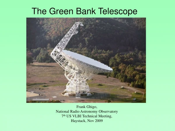
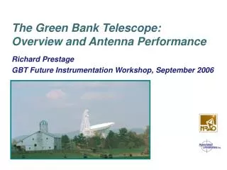
The Green Bank Telescope: Overview and Antenna Performance. Richard Prestage GBT Future Instrumentation Workshop, September 2006. Overview. General GBT overview (10 mins) GBT antenna performance (20 mins). GBT Size. GBT optics. 100 x 110 m section of a parent parabola 208 m in diameter

E N D
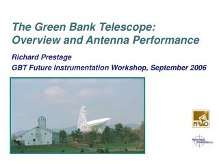
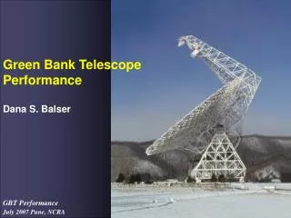
The Green Bank Telescope:Overview and Antenna Performance Richard Prestage GBT Future Instrumentation Workshop, September 2006
Overview • General GBT overview (10 mins) • GBT antenna performance (20 mins)
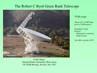
GBT optics • 100 x 110 m section of a parent parabola 208 m in diameter • Cantilevered feed arm is at focus of the parent parabola
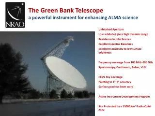
GBT Capabilities • Extremely powerful, versatile, general purpose single-dish radio telescope. • Large diameter filled aperture provides unique combination of high sensitivity and resolution for point sources plus high surface-brightness sensitivity for faint extended sources. • Offset optics provides an extremely clean beam at all frequencies. • Wide field of view (10’ diameter FOV for Gregorian focus). • Frequency coverage 290 MHz – 50 GHz (now), 115 GHz (future). • Extensive suite of instrumentation including spectral line, continuum, pulsar, high-time resolution, VLBI and radar backends. • Well set up to accept visitor backends (interfacing to existing IF), other options (e,g, visitor receivers) possible with appropriate advance planning and agreement. • (Comparatively) low RFI environment due to location in National Radio Quiet Zone. Allows unique HI and pulsar observations. • Flexible python-based scripting interface allows possibility to develop extremely effective observing strategies (e.g. flexible scanning patterns). • Remote observing available now, dynamic scheduling under development.
Azimuth Track Fix • Track will be replaced in the summer of 2007. Goal is to restore the 20 year service life of the components. Work includes: • Replace base plates with higher grade material. • New, thicker wear plates from higher grade material. Stagger joints with base plate joints. • Thickness of the grout will be reduced to keep the telescope at the same level. • Epoxy grout instead of dry-pack grout. • Teflon shim between plates. • Tensioned thru-bolting to replace screws. • Outage April 30 to August 3, followed by one month re-commissioning / shared-risk observing period.
Azimuth Track Fix Old Track Section New Bolts Extend Through Both Plates Transition Section Joints Aligned Vertically – Weak Design Screws close to Wheel Path Experienced Fatigue • New Wear Plates • Better Suited Material • Balanced Joint Design • Joints staggered with • Base Plate Joints New Higher Strength Base Plates
Precision Telescope Control System • Goal of the PTCS project is to deliver 3mm operation. • Includes instrumentation, servos (existing), algorithm and control system design, implementation. • As delivered antenna => 15GHz operation (Fall 2001) • Active surface and initial pointing/focus tracking model => 26GHz operation (Spring 2003) • PTCS project initiated November 2002: • Initial 50GHz operation: Fall 2003 • Routine 50 GHz operation: Spring 2006 • Project largely on hold since Spring 2005, but now fully ramping up again.
Summary of Requirements (GHz)
Performance – Tracking Half-power in Azimuth Half-power in Elevation
Power Spectrum Servo resonance 0.28 Hz
Performance – Summary Benign Conditions: (1) Exclude 10:00 18:00 (2) Wind < 3.0 m/s Blind Pointing: (1 point/focus) Offset Pointing: (90 min) Continuous Tracking: (30 min)
“out-of-focus” holography • Hills, Richer, & Nikolic (Cavendish Astrophysics, Cambridge) have proposed a new technique for phase-retrieval holography. It differs from “traditional” phase-retrieval holography in three ways: • It describes the antenna surface in terms of Zernike polynomials and solves for their coefficients, thus reducing the number of free parameters • It uses modern minimization algorithms to fit for the coefficients • It recognizes that defocusing can be used to lower the S/N requirements for the beam maps
Technique • Make three Nyquist-sampled beam maps, one in focus, one each ~ five wavelengths radial defocus • Model surface errors (phase errors) as combinations of low-order Zernike polynomials. Perform forward transform to predict observed beam maps (correctly accounting for phase effects of defocus) • Sample model map at locations of actual maps (no need for regridding) • Adjust coefficients to minimize difference between model and actual beam maps.
Surface Accuracy • Large scale gravitational errors corrected by “OOF” holography. • Benign night-time rms ~ 350µm • Efficiencies: 43 GHz: ηS = 0.67 ηA = 0.47 90 GHz: ηS = 0.2 ηA = 0.15 • Now dominated by panel-panel errors (night-time), thermal gradients (day-time)
Pointing Requirements Condon (2003)
Focus Requirements Srikanth (1990) Condon (2003)
Surface Error Requirements Ruze formula: ε = rms surface error ηp = exp[(-4πε/λ)2] “pedestal” θp ~ Dθ/L ηa down by 3dB for ε = λ/16 “acceptable” performance ε = λ/4π