Download
1 / 24
240 likes | 485 Vues
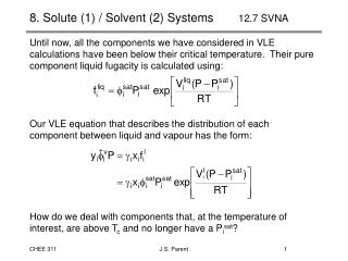
8. Solute (1) / Solvent (2) Systems 12.7 SVNA. Until now, all the components we have considered in VLE calculations have been below their critical temperature. Their pure component liquid fugacity is calculated using:

E N D
8. Solute (1) / Solvent (2) Systems 12.7 SVNA • Until now, all the components we have considered in VLE calculations have been below their critical temperature. Their pure component liquid fugacity is calculated using: • Our VLE equation that describes the distribution of each component between liquid and vapour has the form: • How do we deal with components that, at the temperature of interest, are above Tc and no longer have a Pisat? J.S. Parent
VLE Above the Critical Point of Pure Components J.S. Parent
Pure Species Fugacity of a Solute • The difficulty in handling a component that is above its critical temperature or simply unstable as a pure liquid is to define a pure component fugacity for the purpose of VLE calculations. • While this component must • have a liquid solution • fugacity, f1l, it does not have • a pure liquid fugacity, f1l at • x1 = 1. • The tangent line at x1=0 is • the Henry’s constant, k1. • It is useful for predicting the • mixture fugacity of a dilute • component, but it cannot • be extrapolated to x1=1 • with any degree of accuracy. J.S. Parent
Pure Component Fugacity of a Solute • The pure component fugacity of a solute is calculated from a combination of Henry’s Law and an activity coefficient model. • Recall that Henry’s Law may be used to represent the mixture fugacity of a minor (xi<0.02) component in a liquid. • defines the Henry’s • constant • and • is accurate as long • as x1 < 0.02 • Unfortunately, we cannot extrapolate the above equation to x1 = 1 to give us the pure component f1. • An activity coefficient model can refine this approach J.S. Parent
Pure Component Fugacity of a Solute • Recall that the activity coefficient is the ratio of the mixture fugacity of a component to its ideal solution fugacity: • At infinite dilution (x10), the activity coefficient becomes: • Since the pure component fugacity is a constant at a given T, we can write this expression as: • Using the definition of the Henry’s Constant, ki, we have: • or 12.34 J.S. Parent
Pure Component Fugacity of a Solute • Equation 12.34 is a rigorous thermodynamic equation, • 12.34 • for the fugacity of a “pure” solute. However, it is evaluated at P2sat (where x1 = 0) and its use requires us to assume that pressure has an insignificant influence on the solute’s fugacity. • To apply 12.34, we require a Henry’s constant for the system at the temperature of interest, ki(T), and an excess Gibbs energy model for the system, also at the T of interest. J.S. Parent
VLE Relationship for a Supercritical Component • Consider a system where one component is above Tc (species 1) and the other component is below Tc (species 2). • The equilibrium relationship for component 2 is unchanged: • or • However, component 1 is handled differently, using a Henry’s constant (k1) and the infinite dilution activity coefficient (1). Both are properties specific to this mixture. • 12.36 J.S. Parent
Solute (1) / Solvent (2) Systems: Example J.S. Parent
9. Phase Stability and Liquid-Liquid Equilibria • Throughout the course we have developed methods of calculating the thermodynamic properties of different systems: • Gibbs energy of pure vapours and liquids • Gibbs energy of ideal and real mixtures • Definition of vapour liquid equilibrium conditions • As we apply these methods, we assume that the phases are stable. • Recall our calculation of the Gibbs energy of a hypothetical liquid while developing Raoult’s law. • In our flash calculations that we calculated Pdew and Pbubble before assuming that two phases exist • A slight extension of the thermodynamic theory covered in CHEE 311 provides us with a means of assessing the stability of a phase. • Answers the question: “Will the system actually exist in the state I have chosen?” J.S. Parent
Phase Stability • A system at equilibrium has minimized the total Gibbs energy. • Under some conditions (relatively low P, high T) it assumes a vapour state • Under others (relatively high P, low T) the system exists as a liquid • Mixtures at specific temperatures and pressures exist as a liquid and vapour in equilibrium • Consider the mixing of two, pure liquids. We can observe two behaviours: • complete miscibility which creates a single liquid phase • partial miscibility which creates two liquid phases • in the extreme case, these phases may be considered completely immiscible. J.S. Parent
+ Stability and the Gibbs Energy of Mixing • We have already discussed the property changes of mixing, in particular the Gibbs energy of mixing. • Before After • GA GB G • nA moles nB moles nA + nB moles • liquid A liquid B of mixture • The Gibbs energy of mixing is defined as: • which in terms of mole fractions becomes: J.S. Parent
Stability and the Gibbs Energy of Mixing • The mixing of liquids changes the Gibbs energy of the system by: • Clearly, this quantity must • be negative if mixing is to • occur, meaning that the • mixed state is lower in • Gibbs energy than the • unmixed state. J.S. Parent
Stability Criterion Based on Gmix • If the system can lower its Gibbs energy by splitting a single liquid phase into two liquids, it will proceed towards this multiphase state. • A criterion for single phase stability can be derived from a knowledge of the composition dependence of Gmix. • For a single phase to be stable at a given temperature, pressure and composition: • Gmix and its first and second derivatives must be continuous functions of x1 • The second derivative of Gmix must satisfy: • 14.5 J.S. Parent
Phase Stability Example: Phenol-Water J.S. Parent
Phase Stability Example: Phenol-Water (25C) J.S. Parent
Liquid-Liquid Equilibrium: Phenol-Water J.S. Parent
9. Liquid Stability 14.1 SVNA • Whether a multi-component liquid system exists as a single liquid or two liquid phases is determined by the stability criterion: • 14.5 • If this condition holds, the liquid is stable. If not, it will split into two (or more) phases. • Substituting Gmix for a binary system, • (A) • we derive an alternate stability criteria based on component 1: • (A) into 14.5 • This quantity must be positive for a liquid to be stable. J.S. Parent
Wilson’s Equation and Liquid Stability • Given our phase stability criterion: • what we require to gauge liquid stability is an activity coefficient model. Wilson’s equation for component 1 of a binary system gives: • 11.17 • Applying our stability criterion to 11.17 yields: • Given that all Wilson’s coefficients Lij are positive, all quantities on the right hand side are greater than zero for all compositions • Wilson’s equation cannot predict liquid instability, and cannot be used for LLE modeling. J.S. Parent
Liquid-Liquid Equilibrium (LLE) SVNA 14.2 J.S. Parent
Liquid-Liquid Equilibrium: Phenol-Water J.S. Parent
Liquid-Liquid Equilibrium Relationships • Two liquid phases (a,b) at equilibrium must have equivalent component mixture fugacities: • In terms of activity coefficients: • If each component can exist as a liquid at the given T,P, the pure component fugacities cancel, leaving us with: • 14.10 • Note that the same activity coefficient expression applies to each phase. J.S. Parent
Liquid-Liquid Equilibrium-NRTL • Consider a binary liquid-liquid system described by the NRTL excess Gibbs energy model. • For phase a, we have: • 11.20 • 11.21 • For phase b, we have: • 11.20 • 11.21 • The activity coefficients of the two liquids are distinguished solely by the mole fractions of the phases to which they apply. J.S. Parent
Liquid-Liquid Equilibrium Calculations • In CHEE 311, we will consider only binary liquid-liquid systems at conditions where the excess Gibbs energy is not influenced by pressure. • The phase rule tells us F=2-p+C • =2-2+2 = 2 degrees of freedom • If T and P are specified, all intensive variables are fixed • For this two-component system we can write the following equilibrium relationships: • and 14.10 • The latter can be stated in terms of component 1, to yield: • and 14.12 • The activity coefficients gia and gib are functions of xia and xib. J.S. Parent
Liquid-Liquid Equilibrium Calculations • Once we establish that a LLE condition exists, we are interested to know the composition of the two phases. • Given T (and P), find the composition of the two liquids. • Start with our equilibrium relationships. • Component 1: • Component 2: • The natural logarithm is usually simpler to solve: • We have two equations, and two • unknowns xia and xib. J.S. Parent