CTC 450
CTC 450. Pumps. http://www.esi-group.com/SimulationSoftware/CFD_ACE/blood.html. Objectives. Ability to simplify pipe systems by use of equivalent pipes (parallel and series) Know what types of pumps are available Ability to develop a pump performance curve

CTC 450
E N D
Presentation Transcript
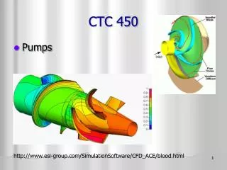
CTC 450 • Pumps http://www.esi-group.com/SimulationSoftware/CFD_ACE/blood.html
Objectives • Ability to simplify pipe systems by use of equivalent pipes (parallel and series) • Know what types of pumps are available • Ability to develop a pump performance curve • Ability to develop a simple system curve
Equivalent Pipes • An imaginary conduit that replaces a section of a real system such that the head losses are identical for the quantity of flow
Equivalent Pipe to Replace Parallel Pipes-Ex 4-19; page 113 • Determine an equivalent pipe 1000’ in length to replace two parallel pipes (8” pipe @ 1000’ and 6” pipe @ 800’) • Assume a head loss (10’) and calculate HGL slopes of both pipes (10’/1000’) and (10’/800’). Using diameters and HGL slopes calculate Q in both pipes from Hazen-Williams nomograph (550 & 290 gpm) • Total Q’s (840 gpm) • Use nomograph w/ HGL slope (10’/1000’) and total Q to get equivalent pipe size (answer=9.4”)
Equivalent Pipe to Replace Serial Pipes • Determine an equivalent pipe 2000’ in length to replace three pipes in series (8” pipe @ 400’ , 9.4” pipe @ 1,000’ and 10” pipe @ 600’) • Assume a flow (500 gpm) and calculate head losses in all 3 pipes from Hazen-Williams equation or nomograph (3.3+3.8+1.6=8.7’ per 2000’) • Determine head losses per 1000’ (4.4’ per 1,000 ft) • Use nomograph w/ calculated head loss and assumed Q to get equivalent pipe size (answer=9.2”)
Pumps • Machines that do work on fluids • Pumps increase the pressure in a pipe, or lift water, or move water • Axial-flow • Flow is parallel to axis • Best suited for low heads and high flows • Radial-flow (centrifugal) • Flow is perpendicular to axis • Best suited for high heads
Pump Performance Curves • Obtained by experimental data and plotted on graphs (usually for a specific pump at a specific rotation speed) • Head versus discharge • Efficiency versus discharge • Shutoff head is the pressure head if discharge is completely stopped (Q=0)
Pump Efficiency • Efficiency is defined as the motor power input divided by the power output • Centrifugal pump efficiency is usually in the range of 60-85%
Variable Speed Pumps • Pumps which can be operated at variable speeds • Have 2 pump curves (high speed and low speed) and pump can operate between the curves
System Head Curves • Accounts for static head and friction losses in the system • Static head (lifting of water to a higher elevation) • Friction losses (increases as the flow increases) • In real systems, outputs are variable and the system head “curve” is actually a “band” • Pump should be operated at the intersection of the system-head curve and the head-discharge curve
System Head Curve Example • See page 108 (Figures 4-14 & 4-15) • Curve 1 – If pump is used to “raise” water from a lower source to a higher tank (outlet 1) • Curve 2 – If pump is used to raise water to a load center (outlet 2) • Actual operation can vary between the curves depending on how much flow is discharging from outlet 1 and 2
System CurvesCurve 1: Pump to StorageCurve 2: Pump to Load What do H1 and H2 represent? How do you calculate the increase in head based on the pumping rate?
Pump & System Head Curves Example Pump operates at A when pumping only to storage Pump operates at B when pumping only to the load Pump operates at C when pumping partly to the storage tank and partly to the load
Example-Discussion of Pumps • Small system • Use 2 constant speed pumps with same capacity • Intermittently pump to tank • Control by fluctuation of water level in tank • Elevated storage maintains pressure in the system
Example-Discussion of Pumps • Large system • Use 3 pumps in parallel (1 as standby) • Operate pumps individually or in combination to meet demand
http://www.armstrongpumps.com/present_newsletter.asp?groupid=1&nlfile=00_00_054http://www.armstrongpumps.com/present_newsletter.asp?groupid=1&nlfile=00_00_054
Pump Operation ScenariosSingle Pump • Constant speed (as flows change the pump pressure changes) • Variable speed (maintains a constant pressure over a wide range of flows by varying the rotational speed of the pump impellor)
Pump Operation Scenarios Multiple Pumps • Multiple pumps – parallel – one as “standby” • Multiple pumps – series – to increase discharge head
Pumps http://www.simerics.com/simulation_gallery.html
Next Lecture • Manning’s Equation (open channel flow) • Rational Method
Midterm • Open Book/Open Notes • Thursday, October 10th (10 am-Noon) • Will cover lectures 1-9 • Chemistry • Biology • Fluid Statics • Buoyancy • Fluid Flow (continuity, storage) • Bernoulli’s/Energy • Friction