Download
1 / 16
170 likes | 793 Vues
Explore Fourier series representation of time functions, Fourier transform properties, examples of transforms, and generalization to non-periodic signals. Learn about basis functions, convergence criteria, Dirichlet conditions, and transforming periodic signals into continuous functions. Delve into Fourier coefficients, transform pairs, and applications through various signal examples.

E N D
Lecture 8: Fourier Series and Fourier Transform • 3. Basis functions (3 lectures): Concept of basis function. Fourier series representation of time functions. Fourier transform and its properties. Examples, transform of simple time functions. • Specific objectives for today: • Examples of Fourier series of periodic functions • Rational and definition of Fourier transform • Examples of Fourier transforms
Lecture 8: Resources • Core material • SaS, O&W, C3.3, 3.4, 4.1, 4.2 • Background material • MIT Lecture 5, Lecture 8 • Note that in this lecture, we’re initially looking at periodic signals which have a Fourier series representation: a discrete set of complex coefficients • However, we’ll generalise this to non-periodic signals that which have a Fourier transform representation: a complex valued function • Fourier series sum becomes a Fourier transform integral
Example 1: Fourier Series sin(w0t) • The fundamental period of sin(w0t) is w0 • By inspection we can write: • So a1 = 1/2j, a-1 = -1/2j and ak = 0 otherwise • The magnitude and angle of the Fourier coefficients are:
Example 1a: Fourier Series sin(w0t) • The Fourier coefficients can also be explicitly evaluated • When k = +1 or –1, the integrals evaluate to T and –T, respectively. Otherwise the coefficients are zero. • Therefore a1 = 1/2j, a-1 = -1/2j
Example 2: Additive Sinusoids • Consider the additive sinusoidal series which has a fundamental frequency w0: • Again, the signal can be directly written as: • The Fourier series coefficients can then be visualised as:
Example 3: Periodic Step Signal • Consider the periodic square wave, illustrated by: • and is defined over one period as: • Fourier coefficients: NB, these coefficients are real
Example 3a: Periodic Step Signal • Instead of plotting both the magnitude and the angle of the complex coefficients, we only need to plot the value of the coefficients. • Note we have an infinite series of non-zero coefficients T=4T1 T=8T1 T=16T1
Convergence of Fourier Series • Not every periodic signal can be represented as an infinite Fourier series, however just about all interesting signals can be (note that the step signal is discontinuous) • The Dirichlet conditions are necessary and sufficient conditions on the signal. • Condition 1. Over any period, x(t) must be absolutely integrable • Condition 2. In any finite interval, x(t) is of bounded variation; that is there is no more than a finite number of maxima and minima during any single period of the signal • Condition 3. In any finite interval of time, there are only a finite number of discontinuities. Further, each of these discontinuities are finite.
Fourier Series to Fourier Transform • For periodic signals, we can represent them as linear combinations of harmonically related complex exponentials • To extend this to non-periodic signals, we need to consider aperiodic signals as periodic signals with infinite period. • As the period becomes infinite, the corresponding frequency components form a continuum and the Fourier series sum becomes an integral (like the derivation of CT convolution) • Instead of looking at the coefficients a harmonically –related Fourier series, we’ll now look at the Fourier transform which is a complex valued function in the frequency domain
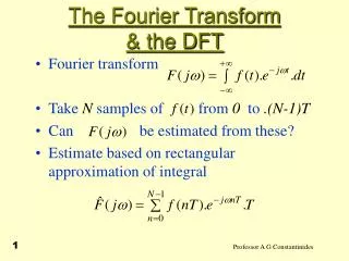
Definition of the Fourier Transform • We will be referring to functions of time and their Fourier transforms. A signal x(t) and its Fourier transform X(jw) are related by the Fourier transform synthesis and analysis equations • and • We will refer to x(t) and X(jw) as a Fourier transform pair with the notation • As previously mentioned, the transform function X() can roughly be thought of as a continuum of the previous coefficients • A similar set of Dirichlet convergence conditions exist for the Fourier transform, as for the Fourier series (T=(- ,))
Example 1: Decaying Exponential • Consider the (non-periodic) signal • Then the Fourier transform is: a = 1
Example 2: Single Rectangular Pulse • Consider the non-periodic rectangular pulse at zero • The Fourier transform is: Note, the values are real T1 = 1
X(jw) w Example 3: Impulse Signal • The Fourier transform of the impulse signal can be calculated as follows: • Therefore, the Fourier transform of the impulse function has a constant contribution for all frequencies
Example 4: Periodic Signals • A periodic signal violates condition 1 of the Dirichlet conditions for the Fourier transform to exist • However, lets consider a Fourier transform which is a single impulse of area 2p at a particular (harmonic) frequency w=w0. • The corresponding signal can be obtained by: • which is a (complex) sinusoidal signal of frequency w0. More generally, when • Then the corresponding (periodic) signal is • The Fourier transform of a periodic signal is a train of impulses at the harmonic frequencies with amplitude 2pak
Lecture 8: Summary • Fourier series and Fourier transform is used to represent periodic and non-periodic signals in the frequency domain, respectively. • Looking at signals in the Fourier domain allows us to understand the frequency response of a system and also to design systems with a particular frequency response, such as filtering out high frequency signals. • You’ll need to complete the exercises to work out how to calculate the Fourier transform (and its inverse) and evaluate the frequency content of a signal
Lecture 8: Exercises • Theory • SaS, O&W, Q4.1-4.4, 4.21 • Matlab • To use the CT Fourier transform, you need to have the symbolic toolbox for Matlab installed. If this is so, try typing: • >> syms t; • >> fourier(cos(t)) • >> fourier(cos(2*t)) • >> fourier(sin(t)) • >> fourier(exp(-t^2)) • Note also that the ifourier() function exists so… • >> ifourier(fourier(cos(t)))