Evolving Binary Image Representations Using Iterated Maps and Genetic Algorithms
20 likes | 134 Vues
This study explores an innovative approach to mapping binary images onto iterated maps through genetic algorithms. By evolving a set of iterated equations from a random pool, we can derive a representation of the image with 100% accuracy. Our findings illustrate the construction and manipulation of chromosomes that facilitate this process, demonstrating how constants, functions, and operands can be effectively represented. By employing metrics like Hausdorff distance for image similarity, we showcase the chaotic nature and potential applications of iterated maps in image representation.

Evolving Binary Image Representations Using Iterated Maps and Genetic Algorithms
E N D
Presentation Transcript
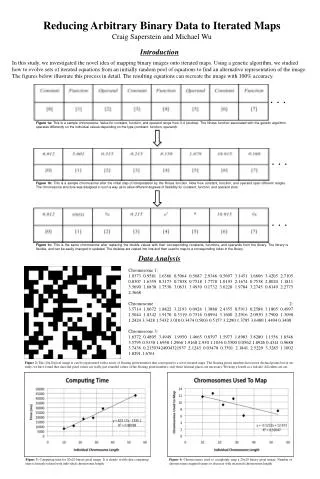
Introduction In this study, we investigated the novel idea of mapping binary images onto iterated maps. Using a genetic algorithm, we studied how to evolve sets of iterated equations from an initially random pool of equations to find an alternative representation of the image. The figures below illustrate this process in detail. The resulting equations can recreate the image with 100% accuracy. . . . Figure 1a: This is a sample chromosome. Value for constant, function, and operand range from 0-4 (double). The fitness function associated with the genetic algorithm operates differently on the individual values depending on the type (constant, function, operand). Reducing Arbitrary Binary Data to Iterated MapsCraig Saperstein and Michael Wu . . . Figure 1b: This is a sample chromosome after the initial step of interpretation by the fitness function. Note how constant, function, and operand span different ranges. The chromosome structure was designed in such a way as to allow different degrees of flexibility for constant, function, and operand slots. . . . Figure 1c: This is the same chromosome after replacing the double values with their corresponding constants, functions, and operands from the library. The library is flexible, and can be easily changed or updated. The doubles are casted into ints and then used to map to a corresponding index in the library. Data Analysis Chromosome 1: 1.0373 0.9581 1.6366 0.5064 0.5687 2.9346 0.5697 3.1451 1.6606 3.4205 2.7105 0.8307 1.6359 0.5173 0.7838 0.7518 1.7778 1.0193 2.1674 0.7538 2.8024 1.1811 3.5690 1.6830 1.7530 3.0631 3.4930 0.1732 3.6228 1.9784 3.2745 0.8149 2.2775 2.3668 Chromosome 2:3.5714 1.0672 1.8822 3.2193 0.0926 1.3888 2.4355 0.5913 0.2588 3.1805 0.4997 1.5044 1.8342 1.9170 0.3319 0.7516 0.0994 3.1600 2.2916 2.0930 3.7900 1.3090 1.2424 3.3428 1.5432 3.010 0.3474 0.5003 0.5157 3.2290 1.3785 3.6480 1.4494 0.3400 Chromosome 3: 1.6372 0.4805 3.4949 1.9950 1.4665 0.8397 1.5973 1.8983 3.8280 1.1556 1.8546 3.5795 0.5330 1.6958 1.2966 1.9168 2.930 1.1036 0.5500 0.0562 1.8926 0.4341 0.9680 3.7436 0.21593424004321937 2.1243 0.03478 0.3501 2.1841 2.5229 3.3285 1.1002 1.8291 1.6761 Figure 2: This 20x20 pixel image is can be represented with a series of floating point numbers that correspond to a set of iterated maps. The floating points numbers have more decimal points but in our study, we have found that since the pixel values are really just rounded values of the floating point numbers, only three decimal places are necessary. We keep a fourth as a failsafe. All others are cut. Figure 3: Computing time for 20x20 binary pixel image. It is clearly visible that computing time is linearly related with individual chromosome length. Figure 4: Chromosomes used to completely map a 20x20 binary pixel image. Number of chromosomes required seems to decrease with increased chromosome length.
Hausdorff Distance Unlike normal functions whose values can be easily obtained given a specific relationship between x and y, iterated equations generally must be iterated to obtain the next value of x and y. While this may sound irksome, if an entire iterated equation is given a modulus, a seemingly simple iterated equation may take on chaotic behavior. This property makes iterated equations very interesting mathematically. Such an equation is generally of the form: Xn+1= F (Xn) where F is known as the mapping function, hence the name iterated maps. To best illustrate the potential of iterated maps, we have included the x and y equations of the standard map below. Xn+1 = [Xn + Ksin(Yn)] mod 2π Yn+1 = [Yn + Xn+1] mod 2π These two equations represent the standard map, where K is a constant whose value can be any real number. This map represents the chaotic behavior of the “kicked rotator”, a stick that is allowed to rotate on one of its axis free of gravitational force and is kicked periodically. This system approximates systems common in accelerator physics. Here, we simply want to evaluate the potential of this image to “change shape”. Below is an image of the standard map with K = 0.893. Varying K results in varying chaotic behavior. This means that iterated equations have the potential to cover a wide range of shapes and images. Iterated Maps There are various metrics of measuring image similarity, including SSIM and PSNR. However, due to the inherent chaotic nature of the iterated maps, we chose to use the Hausdorff distance. SSIM and PSNR take into the similarity of two entire images, while the Hausdorff distance will compare the active parts of one image with another image. For example, given two sets, A and B, the Hausdorff distance from A to B is the maximum distance any point in A is from B. Formally the Hausdorff distance is defined as: H (A, B) = max(h(A, B), h(B, A)) where h(A, B) = max min ||a – b|| A2 A1 B3 B1 d2 B2 d1 Figure 7: The Hausdorff distance, H(A, B), is d1. If H(A, B) is zero, it means that the points in set A can be found in set B. The Hausdorff distance is a maximum minimum function. In the diagram shown here with sets A and B, the Hausdorff distance can be calculated by recording the minimum distance from each point in set A to set B and taking the maximum of those distances. d1and d2 are the minimum distances from A1 and A2 respectively to a point belonging in set B. Here the Hausdorff distance would be equal to d1 because it is larger than d2. Applications to Other File Types For purposes of our algorithm, images were treated as lists of binary data. Since every data type can be represented as a list of binary data, it is possible to apply our algorithm to reduce anything, including its output, to a set of iterated maps which take up less space. Figure 5: Standard Map with K value of 0.9. As K increases, the Standard Map becomes more chaotic. Conclusions Our work has shown that it is possible to represent arbitrary binary data with a set of iterated maps. A genetic algorithm was tried, but a deterministic method that minimized the Hausdorff distance error function proved to be much faster. The numerical methods used were not optimal for chaotic root finding, so the development of a generalized chaotic root finding algorithm would drastically increase the speed of the algorithm. Applications of transforming data to chaotic maps exist in compression, encryption, modeling, or any field that involves finding complicated patterns among data. Figure 6: Standard Map with K value of 1.4. As K increases, the Standard Map becomes more chaotic. Library References [1] M.F Barnsley and A.D Sloan, Fractal image compression, Proc. Scientific Data Compression Workshop, May 1988, Pages 351–365. [2] J. Blanck, Efficient exact computation of iterated maps, Journal of Logic and Algebraic Programming, Volume 64, Issue 1, July 2005, Pages 41-59, ISSN 1567-8326. [3] A.E. Jacquin, Fractal image coding based on a theory of iterated contractive image transformations, SPIE Vol. 1360 Visual Communications and Image Processing '90, Pages 227–239. [4] Guojun Lu, Fractal image compression, Signal Processing: Image Communication, Volume 5, Issue 4, October 1993, Pages 327-343, ISSN 0923-5965. [5] G Lu, Advances in digital image compression techniques, Comput. Comm.Volume 16, Issue 4, April 1993, Pages 202–214 [6] Meffert, Klaus et al.: JGAP - Java Genetic Algorithms and Genetic Programming Package. URL: http://jgap.sf.net [7] N.W. Murray, Critical function for the standard map, Physica D: Nonlinear Phenomena, Volume 52, Issues 2-3, September 1991, Pages 220-245, ISSN 0167-2789. [8] D. Vidya, Ranjani Parthasarathy, T. C. Bina, N. G. Swaroopa, Architecture for fractal image compression, Journal of Systems Architecture, Volume 46, Issue 14, December 2000, Pages 1275-1291, ISSN 1383-7621. [9] Lei Wang, Licheng Jiao, Jiaji Wu, Guangming Shi, Yanjun Gong, Lossy-to-lossless image compression based on multiplier-less reversible integer time domain lapped transform, Signal Processing: Image Communication, Volume 25, Issue 8, September 2010, Pages 622-632, ISSN 0923-5965. [10] Yasmin H. Said, On Genetic Algorithms and their Applications, In: C.R. Rao, E.J. Wegman and J.L. Solka, Editor(s), Elsevier, 2005, Volume 24, Data Mining and Data Visualization, Pages 359-390, ISSN 0169-7161. *All images and diagrams presented here were created by Craig Saperstein and Michael Wu Table 1: The double genes in the chromosome are cast to integers. This chart maps particular indices to specific functions and operands. Our library is used to determine which indices map to which constant, function, and operands. x represents the input. The first input is always the initial starting point. This initial point does not need to be an integer (pixel coordinate). To speed up evolution of the chromosomes, we generally choose a starting point such as (0.001, 0.001) that is close to the origin.