EARTHQUAKE SCIENCE-ENGINEERING INTERFACE: STRUCTURAL ENGINEERING RESEARCH PERSPECTIVE
Explore the intersection of earth science and structural engineering in examining seismic hazards, assessing structures, and developing efficient methodologies. Learn from best practices and research perspectives in seismic design and analysis.

EARTHQUAKE SCIENCE-ENGINEERING INTERFACE: STRUCTURAL ENGINEERING RESEARCH PERSPECTIVE
E N D
Presentation Transcript
EARTHQUAKE SCIENCE-ENGINEERING INTERFACE: STRUCTURAL ENGINEERING RESEARCH PERSPECTIVE Allin Cornell Stanford University SCEC WORKSHOP Oakland, CA October, 2003
Objective • λC = mean annual rate of State C, e.g., collapse • Two Steps: earth science and structural engineering: λC = ∫PC(X) dλ(X) • Where X = Vector Describing Interface
“Best” Case • X = {A1(t1), A2(t2), …Ai(ti)..} for all ti = i∆t , i = 1, 2, …n i.e., an accelerogram ·dλ(x) = mean annual rate of observing a “specific” accelerogram, e.g., a(ti) < A(ti) <a(ti) + da for all ∙Then engineer finds PC(x) for all x ∙ Integrate
Current Best “Practice” (or Research for Practice) • λC = mean annual rate of State C, e.g., collapse • Two Steps: earth science and structural engineering: λC = ∫PC(IM) dλ(IM) • IM = Scalar “Intensity Measure”, e.g., PGA or Sa1 • λ(IM) from PSHA • PC(IM) found from “random sample” of accelerograms = fraction of cases leading to C
Current Best Seismology Practice*: ·Disaggregate PSHA at Sa1 at po, say, 2% in 50 years, by M and R: fM,R|Sa. Repeat for several levels, Sa11, Sa12, … · For Each Level Select Sample of Records: from a “bin” near mean (or mode) M and R. Same faulting style, hanging/foot wall, soil type, … · Scale the records to the UHS (in some way, e.g., to the Sa(T1)). *DOE, NRC, PEER, … e.g., see R.K. McGuire: “... Closing the Loop”( BSSA, 1996+/-); Kramer (Text book; 1996 +/-); Stewart et al. (PEER Report, 2002)
105 105 105 105 105 106 157 241 241 241 Seismic Design Assessment of RC Structures. (Holiday Inn Hotel in Van Nuys) • Beam Column Model with Stiffness • and Strength Degradation in Shear and Flexure • using DRAIN2D-UW by J. Pincheira et al.
Multiple Stripe Analysis C • The Statistical Parameters of the “Stripes” are Used to Estimate the Median and Dispersion as a Function of the Spectral Acceleration, Sa1.
Best “Research-for-Practice” (Cont’d) : • Analysis: λC = ∫PC(IM) dλ(IM) ≈ ∑PC(IMk) ∆ λ(IMk) • Purely Structural Engineering Research Questions: • Accuracy of Numerical Models • Computational Efficiency
Best “Research-for-Practice”: • Analysis: λC = ∫PC(IM) dλ(IM) ≈ ∑PC(IMk) ∆ λ(IMk) ·Interface Questions: What are good choices for IM? Efficient? Sufficient? How does one obtain λ(IM) ? How does one do this transparently, easily and practically?
BETTER SCALAR IM? More Efficient? IM = Sa1 IM = g(Sd-inelastic; Sa2) (Luco, 2002) • when IM1I&2E is employed in lieu of IM1E, (0.17/0.44)2 ≈ 1/7 the number of earthquake records and NDA's are needed to estimate a with the same degree of precision
Sa MAGNITUDE DRIFT Sa Van Nuys Transverse Frame: Pinchiera Degrading Strength Model; T = 0.8 sec. 60 PEER records as recorded 5.3<M<7.3.
DRIFT MAGNITUDE Residual-residual plot: drift versus magnitude (given Sa) for Van Nuys. (Ductility range: 0.3 to 6) (60 PEER records, as recorded.)
DRIFT MAGNITUDE Residual-residual plot: drift versus magnitude (given Sa) of a very short period (0.1 sec) SDOF bilinear system. (Ductility range 1to 20.) (47 PEER records, as recorded.)
DRIFT MAGNITUDE Residual-residual plot: drift versus magnitude (given Sa) for 4-second, fracturing-connection model of SAC LA20. Records scaled by 3. Ductility range: mostly 0.5 to 5
What Can Be Done That is Still Better? • Scalar to (Compact) Vector IM • Interface Issues: What vector? How to find λ (IM)? • Examples: {Sa1, M}, {Sa1, Sa2}, … ·PSHA: λ(Sa1, M) = λ(Sa1) f(M| Sa1) (from “Deagg”) λ(Sa1, Sa2) Requires Vector PSHA (SCEC project)
Vector-Based Response Prediction Vector-Valued PSHA
Future Interface Needs • Engineers: • Need to identify “good” scalar IMs and IM vectors. • In-house issues: what’s “wrong” with current candidates? When? Why? How to fix? • How to make fast and easy, i.e., professionally useful.
Future Interface Needs (con’t) • Help from Earth scientists: Guidance (e.g., what changes frequency content? Non-”random” phasing? ) · Earth Science problems:How likely is it? λ(X) • λ(X) = ∫P(X \ Y) dλ(Y) • X = ground motion variables (ground motion prediction: empirical, synthetic) • Y = source variables (e.g., RELM)
Future Needs(Cont’d) • Especially λ(X) for “bad” values of X (Or IM). ·Some Special Problems: Nonlinear Soils, Strong Directivity, Aftershocks, Spatial Fields of X.
DRIFT MAGNITUDE Residual-residual plot: drift versus magnitude (given Sa) for 4-second, fracturing-connection model of SACLA20. Ductility range: 0.2 to 1.5. Same records.
Non-Linear MDOF Conclusion: (Given Sa(T1) level) the median (displacement) EDP is apparently independent of event parameters such as M, R, …*. Implications: (1) the record set used need not be selected carefully selected to match these parameters to those relevant to the site and structure. Comments: Same conclusion found for transverse components. More periods and backbones and EDPs deserve testing to test the limits of applicability of this illustration. *Provisos: Magnitudes not too low relative to general range of usual interest; no directivity or shallow, soft soil issues.