Download
1 / 24
240 likes | 261 Vues
Explore detailed analysis to improve call center operations, considering variability, resources, and operating procedures. Learn how to analyze demand and arrival processes effectively.

E N D
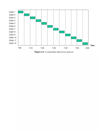
Caller 1 Caller 2 Caller 3 Caller 4 Caller 5 Caller 6 Caller 7 Caller 8 Caller 9 Caller 10 Caller 11 Caller 12 Time 7:00 7:10 7:20 7:30 7:40 7:50 8:00 Figure 6.1: A somewhat odd service process
Caller 1 Caller 3 Caller 5 Caller 7 Caller 9 Caller 11 Arrival Time Service Time Caller 2 Caller 4 Caller 6 Caller 8 Caller 10 Caller 12 Caller 1 0 5 Time 2 7 6 3 9 7 7:00 7:10 7:20 7:30 7:40 7:50 8:00 4 12 6 5 18 5 6 22 2 3 7 25 4 2 8 30 3 Number of cases 9 36 4 1 10 45 2 11 51 2 0 2 min. 3 min. 4 min. 5 min. 6 min. 7 min. 12 55 3 Service times Figure 6.2.: Data gathered at a call center
Caller 1 Caller 2 Caller 3 Caller 4 Caller 5 Caller 6 Caller 7 Caller 8 Caller 9 Caller 10 Caller 11 Caller 12 Service time Wait time 7:00 7:10 7:20 7:30 7:40 7:50 8:00 Inventory (Callers on hold) 5 4 3 2 1 0 7:00 7:10 7:20 7:30 7:40 7:50 8:00 Time Figure 6.3.: Detailed analysis of call center
Activity times: • Inherent variation • Lack of operating procedures • Quality (scrap / rework) Processing Buffer • Input: • Random arrivals (randomness is the rule, not the exception) • Incoming quality • Product Mix • Resources: • Breakdowns / Maintenance • Operator absence • Set-up times • Routes: • Variable routing • Dedicated machines Figure 6.4.: Variability and where it comes from
Arrival Time, ATi Call Inter-Arrival Time, IAi=ATi+1 -ATi 1 6:00:29 Call 1 Call 2 Call 3 Call 4 Call 5 Call 6 Call 7 00:23 2 6:00:52 01:24 3 6:02:16 00:34 4 6:02:50 02:24 5 6:05:14 6:00 6:01 6:02 6:03 6:04 6:05 6:06 Time 00:36 6 6:05:50 00:38 7 6:06:28 IA1 IA2 IA3 IA4 IA5 IA6 Figure 6.5.: The concept of inter-arrival times
Number of customers Number of customers Per 15 minutes Per 15 minutes 160 160 140 140 120 120 100 100 80 80 60 60 40 40 20 20 0 0 Time Time 0:15 0:15 2:00 2:00 3:45 3:45 5:30 5:30 7:15 7:15 9:00 9:00 10:45 10:45 12:30 12:30 14:15 14:15 16:00 16:00 17:45 17:45 19:30 19:30 21:15 21:15 23:00 23:00 : Seasonality over the course of a day : Seasonality over the course of a day Figure 6.6
Cumulative Customers Cumulative Customers 70 700 60 600 50 500 Expected arrivalsif stationary 40 400 30 300 20 200 Actual, cumulative arrivals 10 100 0 0 0 0 6:00:00 6:00:00 6:00:00 7:00:00 7:00:00 7:00:00 8:00:00 8:00:00 8:00:00 9:00:00 9:00:00 9:00:00 10:00:00 10:00:00 10:00:00 7:15:00 7:15:00 7:18:00 7:18:00 7:21:00 7:21:00 7:24:00 7:24:00 7:27:00 7:27:00 7:30:00 7:30:00 Time Time Figure 6.7.: Test for stationary arrivals Test for stationary arrivals
100 1 90 80 0.8 70 60 0.6 Number of calls with given duration t 50 Probability{Interarrival time t} 40 0.4 30 20 0.2 10 0 0 time 0 1 2 3 0.8 1.2 1.6 2.8 3.2 0.2 0.4 0.6 1.4 1.8 2.2 2.4 2.6 Duration t Figure 6.8.: Distribution function of the exponential distribution (left) and an example of a histogram (right)
Distribution Function Distribution Function 1 1 0.8 0.8 Exponential distribution Exponential distribution 0.6 0.6 0.4 0.4 Empirical distribution Empirical distribution (individual points) (individual points) 0.2 0.2 Inter Inter - - arrival time arrival time 0 0 0:00:00 0:00:00 0:00:09 0:00:09 0:00:17 0:00:17 0:00:26 0:00:26 0:00:35 0:00:35 0:00:43 0:00:43 0:00:52 0:00:52 0:01:00 0:01:00 0:01:09 0:01:09 Figure 6.9: Empirical vs. exponential distribution for inter-arrival times
Stationary Arrivals? YES NO Exponentially distributed inter-arrival times? Break arrival process up into smaller time intervals YES NO • Compute a: average interarrival time • CVa=1 • All results of chapters 6 and 7 apply • Compute a: average interarrival time • CVa= St.dev. of interarrival times / a • All results of chapter 6 apply • Results of chapter 7 do not apply, require simulation or more complicated models Figure 6.10: How to analyze a demand / arrival process?
800 Frequency 600 400 200 Std. Dev = 141.46 Call durations [seconds] Mean = 127.2 N = 2061.00 0 0 100 200 300 400 500 600 700 800 900 1000 Figure 6.11: Service times in call center A
Call duration[minutes] 2.5 2 1.5 1 0.5 0 Week-end averages Week-day averages Time of the day 0:00 23:00 Figure 6.12: Average call durations: week-day vs. week-end
Inflow Outflow Entry to system Begin Service Departure Figure 6.13.: A simple process with one queue and one server
Inventory waiting Iq Inventory in service Ip Inflow Outflow Entry to system Begin Service Departure Waiting Time Tq Service Time p Flow Time T=Tq+p Figure 6.14.: A simple process with one queue and one server
Inflow Outflow Departure Entry to system Begin Service Figure 6.15.: A process with one queue and multiple, parallel servers
Inventory in the system I=Iq+ Ip Inventory in service Ip Inventory waiting Iq Outflow Inflow Entry to system Begin Service Departure Waiting Time Tq Service Time p Flow Time T=Tq+p Figure 6.16.: Summary of key performance measures
Fraction of customerswho have to wait xseconds or less 1 Waiting times for those customers who do not get served immediately 0.8 0.6 Fraction of customers who get served without waiting at all 0.4 0.2 0 0 50 100 150 200 Waiting time [seconds] Figure 6.17: Empirical distribution of waiting times at Anser
Call center Answered Calls Incoming calls Sales reps processing calls Calls on Hold Blocked calls (busy signal) Abandoned calls (tired of waiting) Financial consequences Holding cost (line charges) Lost goodwill Lost throughput (abandoned) Cost of capacity Lost throughput Lost goodwill Revenue Figure 6.18: Economic consequences of waiting
Number ofCSRs Number of customers Number of customers Per 15 minutes Per 15 minutes 160 160 17 16 15 14 13 12 11 10 9 8 7 6 5 4 3 2 1 140 140 120 120 100 100 80 80 60 60 40 40 20 20 0 0 Time Time 0:15 0:15 2:00 2:00 3:45 3:45 5:30 5:30 7:15 7:15 9:00 9:00 10:45 10:45 12:30 12:30 14:15 14:15 16:00 16:00 17:45 17:45 19:30 19:30 21:15 21:15 23:00 23:00 Figure 6.19 : Staffing and incoming calls over the course of a day Number of customers Number of customers Number ofCSRs Per 15 minutes Per 15 minutes 160 160 17 16 15 14 13 12 11 10 9 8 7 6 5 4 3 2 1 140 140 120 120 100 100 80 80 60 60 40 40 20 20 0 0 Time Time 0:15 0:15 2:00 2:00 3:45 3:45 5:30 5:30 7:15 7:15 9:00 9:00 10:45 10:45 12:30 12:30 14:15 14:15 16:00 16:00 17:45 17:45 19:30 19:30 21:15 21:15 23:00 23:00
Independent Resources 2x(m=1) Pooled Resources (m=2) Figure 6.20.: The concept of pooling
70.00 Waiting Time Tq [sec] m=1 60.00 50.00 40.00 m=2 30.00 20.00 m=5 10.00 m=10 0.00 Utilization u 60% 65% 70% 75% 80% 85% 90% 95% Figure 6.21: How pooling can reduce waiting time
A A C C B B Service times: A: 9 minutesB: 10 minutesC: 4 minutesD: 8 minutes D D 4 min. 9 min. 19 min. 12 min. 23 min. 21 min. Total wait time: 9+19+23=51min Total wait time: 4+12+21=37 min Figure 6.22: The shortest processing time (SPT) rule (used in the right case)
Call durations 2:00 min. Operator KB short Operator NN 2:30 min. Operator BJ 3:00 min. Operator BK 3:30 min. Operator NJ 4:00 min. long 4:30 min. Low courtesy High courtesy Courtesy / Friendliness (qualitative information) Figure 6.23: Operator performance concerning speed and courtesy
Responsiveness System improvement(e.g. pooling of resources) High Increase staff(lower utilization) Responsive process with high costs Reduce staff(higher utilization) Now Low cost process with low responsiveness Frontier reflecting current process Low High perunit costs(low utilization) Low perunit costs(high utilization) Efficiency Figure 6.24: Balancing efficiency with responsiveness