Download
1 / 82
910 likes | 1.28k Vues
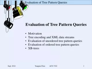
Evaluation of Tree Pattern Queries. Motivation Tree encoding and XML data streams Evaluation of unordered tree pattern queries Evaluation of ordered tree pattern queries XB-trees. Motivation. Efficient method to evaluate XPath expression queries – XML query processing.

E N D
Evaluation of Tree Pattern Queries • Motivation • Tree encoding and XML data streams • Evaluation of unordered tree pattern queries • Evaluation of ordered tree pattern queries • XB-trees Yangjun Chen ACS-7102
Motivation • Efficient method to evaluate XPath expression queries – XML query processing a tree pattern query XML documents Yangjun Chen ACS-7102
P S B N I I L L N Houston Winnipeg Y-Chen Dell M N I N IBM Part#1 Part#2 M Intel Motivation Document: <Purchase> <Seller> <Name>dell</Name> <Item> <Manufacturer>IBM</Manufacturer> <Name>part#1</Name> <Item> <Manufacturer>Intel</Manufacturer> </Item> </Item> <Item> <Name>Part#2</Name> </Item> <Location>Houston</Location> </Seller> <Buyer> <Location>Winnipeg</Location> <Name>Y-Chen</Name> </Buyer> </Purchase> Yangjun Chen ACS-7102
P S B N I I L L N Houston Winnipeg Y-Chen Dell M N I N IBM Part#1 Part#2 M Intel Motivation Document: Query – XPath expressions: Q1: /Purchase[Seller[Loc=‘Boston’]]/ Buyer[Loc = ‘New York’] Purchase Buyer Seller Location Location ‘Winnipeg’ ‘Houston’ Q2: /Purchase//Item[Manufacturer = ‘Intel’] Buyer d-edge: ancestor- descendant relationship Item Manufacturer c-edge: parent-child relationship ‘Intel’ Yangjun Chen ACS-7102
Tree Encoding • Let T be a document tree. We associate each node v in T with a • quadruple (DocId, LeftPos, RightPos, LevelNum),denoted as(v), • where • DocId is the document identifier; • LeftPos and RightPos are generated by counting word • numbers from the beginning of the document until the start • and end of the element, respectively; and • LevelNum is the nesting depth of the element in the • document. • By using such a data structure, the structural relationship between • the nodes in an XML database can be simply determined. Yangjun Chen ACS-7102
<A> <B> <C>string</C> <B> <C>string</C> <C>string</C> <D>string</D> </B> </B> <B> string </B> </A> T: (1, 1, 11, 1) A v1 (1, 10, 10, 2) v2 B B v8 (1, 2, 9, 2) (1, 4, 8, 3) v3 C B v4 (1, 3, 3, 3) (1, 7, 7, 4) v5 C v6 C v7 D (1, 5, 5, 4) (1, 6, 6, 4) DocId LeftPos RightPos LevelNum Yangjun Chen ACS-7102
Tree Encoding • ancestor-descendant: a node v1 associated with (d1, l1, r1, ln1) • is an ancestor of another node v2 with (d2, l2, r2, ln2) iff • d1 = d2, l1 < l2, and r1 > r2. • parent-child: a node v1 associated with (d1, l1, r1, ln1) is the • parent of another node v2 with (d2, l2, r2, ln2) iff d1 = d2, • l1 < l2, r1 > r2, and ln2 = ln1 + 1. • from left to right: a node v1 associated with (d1, l1, r1, ln1) is to • the left of another node v2 with (d2, l2, r2, ln2) iff d1 = d2, • r1 < l2. • . Yangjun Chen ACS-7102
(1, 1, 11, 1) A v1 (1, 2, 9, 2) (1, 10, 10, 2) v2 B B v8 (1, 4, 8, 3) v3 C B v4 (1, 3, 3, 3) (1, 7, 7, 4) v5 C v6 C v7 D (1, 5, 5, 4) (1, 6, 6, 4) C: (1, 3, 3, 3) (1, 5, 5, 4) (1, 6, 6, 4) A: (1, 1, 11, 1) B: (1, 2, 9, 2) (1, 4, 8, 3) (1, 10, 10, 2) D: (1, 7, 7, 4) Data Streams T: The data streams are sorted by (DocID, LeftPos). Yangjun Chen ACS-7102
Tree Pattern queries XPath:/A[//B[//C]/C]//B (1, 2, 9, 2) (1, 4, 8, 3) (1, 10, 10, 2) Q: A q1 {v1} q2 B B q5 {v2, v4, v8} {v2, v4, v8} q3 C C q4 {v3, v5, v6} {v3, v5, v6} descendant edge (//-edge, uv) child edge (/-edge, uv) Yangjun Chen ACS-7102
T: (1, 1, 11, 1) A v1 (1, 2, 9, 2) (1, 10, 10, 2) v2 B B v8 (1, 4, 8, 3) v3 C B v4 (1, 3, 3, 3) (1, 6, 6, 4) v5 C v6 C (1, 5, 5, 4) Data Streams – B(q)’s B(q1): (1, 1, 11, 1) v1 B({q2, q5}): (1, 2, 9, 2) v2 (1, 4, 8, 3) v4 (1, 10, 10, 2) v8 B({q3,q4}): (1, 3, 3, 3) v3 (1, 5, 5, 4) v5 (1, 6, 6, 4) v6 The data streams are sorted by (DocID, LeftPos). Yangjun Chen ACS-7102
Unordered Tree Matching Definition An embedding of a tree pattern Q into an XML document T is a mapping f: Q T, from the nodes of Q to the nodes of T, which satisfies the following conditions: • Preserve node type: For each u Q, u and f(u) are of the same • tag, (or more generally, u’s label is the same as f(u)’s label.) • Preserve ancestor/descendant-parent/child relationships: If uv • in Q, then f(v) is a child of f(u) in T; if uv in Q, then f(v) is a • descendant of f(u) in T. A v1 A q1 T: Q: v2 B B v8 q2 B D q3 v3 C B v4 C v5 v6 C v7 D Yangjun Chen ACS-7102
T: (1, 1, 11, 1) A v1 (1, 2, 9, 2) (1, 10, 10, 2) v2 B B v8 (1, 4, 8, 3) v3 C B v4 (1, 3, 3, 3) (1, 6, 6, 4) v5 C v6 C (1, 5, 5, 4) Data Stream Transformation • Note that iterating through the stream nodes in sorted order of • their LeftPos values corresponds to access of document nodes • in preorder. • We can transform the data streams so that the quadruples sorted • by RightPos values. (Our algorithm needs to access the data • stream in this way.) T: (1, 1, 11, 1) A v1 (1, 2, 9, 2) (1, 10, 10, 2) v2 B B v8 (1, 4, 8, 3) v3 C B v4 (1, 3, 3, 3) (1, 6, 6, 4) v5 C v6 C (1, 5, 5, 4) Yangjun Chen ACS-7102
T: (1, 1, 11, 1) A v1 (1, 2, 9, 2) (1, 10, 10, 2) v2 B B v8 (1, 4, 8, 3) v3 C B v4 (1, 3, 3, 3) (1, 6, 6, 4) v5 C v6 C (1, 5, 5, 4) Data Streams – L(q)’s L(q1): (1, 1, 11, 1) v2 L({q2, q5}): (1, 4, 8, 3) v4 (1, 2, 9, 2) v2 (1, 10, 10, 2) v8 L(q3,q4): (1, 3, 3, 3) v3 (1, 5, 5, 4) v5 (1, 6, 6, 4) v6 The data streams are sorted by (DocID, RightPos). Yangjun Chen ACS-7102
Data Stream Transformation • We maintain a global stack STto make a transformation of data • streams using the following algorithm. • In ST, each entry is a pair (q, v) with q Q, v T (v is • represented by its quadruple) and label(v) = label(q). ST: q (d, l, r, ln) Yangjun Chen ACS-7102
B({q2, q5}) - B: (1, 2, 9, 2) v2 (1, 4, 8, 3) v4 (1, 10, 10, 2) v8 B(q1) - A: (1, 1, 11, 1) v1 B({q3,q4}) -C: (1, 3, 3, 3) v3 (1, 5, 5, 4) v5 (1, 6, 6, 4) v6 B( ) - D: (1, 7, 7, 4) v6 • Algorithmstream-transformation(B(qi)’s) • input: all data streams B(qi)’s, each sorted by LeftPos. • output: new data streams L(qi)’s, each sorted by RightPos. • begin • 1. repeat until each B(qi) becomes empty • 2. { identify qi such that the first element v of B(qi) is of • the minimal LeftPos value; remove v from B(qi); • 3. whileST is not empty and ST.top is not v’s ancestordo • 4. {x ST.pop(); Let x = (qj, u); • 5. put u at the end of L(qi); • 6. } • 7. ST.push(qi, v); • } • Pop out all the remaining elements in ST and insert them into the • corresponding L(qi)’s; • end Yangjun Chen ACS-7102
q3 v3 q2v2 q1v1 • In the above algorithm, ST is used to keep all the nodes on a path • until we meet a node v that is not a descendant of ST.top. • Then, we pop up all those nodes that are not v’s ancestor; put them • at the end of the corresponding L(qi)’s (see lines 3 - 4), and push v • into ST (see line 7), where L(qi) is another datastream created for • qi, sorted by (DocID, RightPos) values. • All the data streams L(qi)’s make up the output of the algorithm. • However, we remark that the popped nodes are in postorder. So • we can directly handle the nodes in this order without explicitly • generating L(qi)’s. T: (1, 1, 11, 1) A v1 B({q2, q5}): (1, 4, 8, 3) v4 (1, 2, 9, 2) v2 (1, 10, 10, 2) v8 B(q1): (1, 1, 11, 1) v1 (1, 2, 9, 2) (1, 10, 10, 2) v2 B B v8 ST: B({q3,q4}): (1, 3, 3, 3) v3 (1, 5, 5, 4) v5 (1, 6, 6, 4) v6 (1, 4, 8, 3) v3 C B v4 (1, 3, 3, 3) (1, 6, 6, 4) (1, 5, 5, 4) v5 C v6 C Yangjun Chen ACS-7102
Matching Subtrees Let T be a tree and v be a node in T with parent node u. Denote by delete(T, v) the tree obtained from T by removing node v. The children of v become ‘descendant’ children of u. B v1 B v1 delete(T, v3) v2 C B v3 v2 C v4 C v5 C v6 D v4 C v5 C v6 D Yangjun Chen ACS-7102
T: A v1 A q1 Q: v2 B B v8 q2 C D q3 v3 C B v4 v5 C v6 C v7 D A v1 v2 C v4 C v5 C v6 D Definition (matching subtrees) A matching subtree T’ of T with respect to a tree pattern Q is a tree obtained by a series of deleting operations to remove any node in T, which does not match any node in Q. a matching subtree: Yangjun Chen ACS-7102
Construction of Matching Subtree from Data Streams • The algorithm given below handles the case when the streams • contain nodes from a single XML document. When the streams • contain nodes from multiple documents, the algorithm is easily • extended to test equality of DocId before manipulating the nodes • in the streams. • It is simply an iterative process to access the nodes in L(Q) one • by one. Here, L(Q) = L(q1) L(q2) … L(qk). q1 = {q1} q2 = {q2, q5} q3 = {q3, q4} L(q1): (1, 1, 11, 1) v2 L(q2): (1, 4, 8, 3) v4 (1, 2, 9, 2) v2 (1, 10, 10, 2) v8 L(q3): (1, 3, 3, 3) v3 (1, 5, 5, 4) v5 (1, 6, 6, 4) v6 Yangjun Chen ACS-7102
Construction of Matching Subtree from Data Streams It is simply an iterative process to access the nodes in L(Q) (= L(q1) L(q2) … L(qk). one by one: • Identify a data stream L(q) with the first element being of the minimal • RightPos value. Choose the first element v of L(q). Remove v from L(q). • Generate a node for v. • If v is not the first node, we do the following: • Let v’ be the node chosen just before v. • - If v’ is not a child (descendant) of v, create a link from v to v’, called • a left-sibling link and denoted as left-sibling(v) = v’. • - If v’ is a child (descendant) of v, we will first create a link from v’ to v, • called a parent link and denoted as parent(v’) = v. Then, we will go • along the left-sibling chain starting from v’ until we meet a node v’’ • which is not a child (descendant) of v. For each encountered node u • except v’’, set parent(u) v. Finally, set left-sibling(v) v’’. Yangjun Chen ACS-7102
v’’ is not a child of v. v v v’ v’ v’’ v’’ … … link to the left sibling In the figure, we show the navigation along a left-sibling chain starting from v’ when we find that v’ is a child (descendant) of v. This process stops whenever we meet v’’, a node that is not a child (descendant) of v. The figure shows that the left-sibling link of v is set to v’’, which is previously pointed to by the left-sibling link of v’s left-most child. Yangjun Chen ACS-7102
L({q2, q5}) - B: (1, 4, 8, 3) v4 (1, 2, 9, 2) v2 (1, 10, 10, 2) v8 L(q1) - A: (1, 1, 11, 1) v1 L({q3,q4}) -C: (1, 3, 3, 3) v3 (1, 5, 5, 4) v5 (1, 6, 6, 4) v6 • Algorithmmatching-tree-construction(L(Q)) (* L(Q) = L(q1) L(q2) … L(qk) *) • input: all data streams L(Q). • output: a matching subtree T’. • begin • repeat until each L(q) in L(Q) becomes empty • { identify q such that the first element v of L(q) is of the minimal RightPos • value; remove v from L(q); • 3. generate node v; • 4. ifv is not the first node created then • 5. {let v’ be the node generated just before v; • 6. ifv’ is not a child (descendant) of v then • 7. left-sibling(v) v’; (*generate a left-sibling link.*) • 8. {v’’v’; wv’; (*v’’ and w are two temporary variables.*) • 9. whilev’’ is a child (descendant) of vdo • 10. {parent(v’’) v; (*generate a parent link. Also, indicate whether v’’ • is a /-child or a //-child.*) • 11. wv’’; v’’left-sibling(v’’); • 12. } • 14. left-sibling(v) v’’; }} • 15. } • end Yangjun Chen ACS-7102
In the above algorithm, for each chosen v from a L(q), a node is • created. • At the same time, a left-sibling link of v is established, pointing to • the node v’ that is generated before v, if v’ is not a child • (descendant) of v (see line 7). • Otherwise, we go into a while-loop to travel along the left-sibling • chain starting from v’ until we meet a node v’’ which is not a child • (descendant) of v. • During the process, a parent link is generated for each node • encountered except v’’. (See lines 9 - 13.) Finally, the left-sibling • link of v is set to be v’’ (see line 14). Yangjun Chen ACS-7102
Example Consider the following data stream L(q)’s: Data Streams – L(q)’s L(q1): (1, 1, 11, 1) v2 L({q2, q5): (1, 4, 8, 3) v4 (1, 2, 9, 2) v2 (1, 10, 10, 2) v8 T: (1, 1, 11, 1) A v1 (1, 2, 9, 2) v2 B B v8 (1, 10, 10, 2) (1, 4, 8, 3) v3 C B v4 (1, 3, 3, 3) L(q3,q4): (1, 3, 3, 3) v3 (1, 5, 5, 4) v5 (1, 6, 6, 4) v6 v5 C v6 C (1, 5, 5, 4) (1, 6, 6, 4) The data streams are sorted by (DocID, RightPos). Yangjun Chen ACS-7102
Example (continued) L(q) = {v1}, L(q’) = {v4, v2, v8}, L(q’’) = {v3, v5, v6}, where q = {q1}, q’ = {q2, q5}, q’’ = {q3, q4}. Applying the above algorithm to the data streams, we generate a series of data structures as shown below. v with the least RightPos: Generated data structure: v3 step 1: v3 L(q1): (1, 1, 11, 1) v2 v3 step 2: v5 v5 L({q2, q5): (1, 4, 8, 3) v4 (1, 2, 9, 2) v2 (1, 10, 10, 2) v8 v3 step 3: v6 v6 v5 v3 L(q3,q4): (1, 3, 3, 3) v3 (1, 5, 5, 4) v5 (1, 6, 6, 4) v6 step 4: v4 v4 v6 v5 Yangjun Chen ACS-7102
v with the least RightPos: Generated data structure: v2 step 5: v2 L(q1): (1, 1, 11, 1) v2 v3 v4 v6 L({q2, q5): (1, 4, 8, 3) v4 (1, 2, 9, 2) v2 (1, 10, 10, 2) v8 v5 v2 v8 step 6: v8 v3 v4 L(q3,q4): (1, 3, 3, 3) v3 (1, 5, 5, 4) v5 (1, 6, 6, 4) v6 v6 v5 v1 step 7: v1 v2 v8 v3 v4 v6 v5 Yangjun Chen ACS-7102
å di i • The time complexity of this process is easy to analyze. • First, we notice that each quadruple in all the data streams is • accessed only once. • Secondly, for each node in T’, all its child nodes will be • visited along a left-sibling chain for a second time. • So we get the total time • O(|D||Q|) + = O(|D||Q|) + O(|T’|) = O(|D||Q|), • where Dis the largest data stream and di represents the outdegree • of node vi in T’. • During the process, for each encountered quadruple, a node v will • be generated. Associated with this node have we at most two links • (a left-sibling link and a parent link). So the used extra space is • bounded by O(|T’|). Yangjun Chen ACS-7102
Proposition1 Let T be a document tree. Let Q be a tree pattern. Let L(Q) = {L(q1), ..., L(ql)} be all the data streams with respect to Q and T, where each qi (1 i l) is a subset of sorted query nodes of Q, which share the same data stream. Algorithm matching-tree-construction(L(Q)) generates the matching subtree T’ of T with respect to Q correctly. Proof. Denote L = |L(q1)| + ... + |L(ql)|. We prove the proposition by induction on L. Basis.When L = 1, the proposition trivially holds. Induction hypothesis.Assume that when L = k, the proposition holds. Induction step.We consider the case when L= k + 1. Assume that all the quadruples in L(Q) are {u1, ..., uk, uk+1} with RightPos(u1) < RightPos(u2) < ... < RightPos(uk) < RightPos(uk+1). Yangjun Chen ACS-7102
The algorithm will first generate a tree structure Tk for {u1, ..., uk}. In terms of the induction hypothesis, Tk is correctly created. It can be a tree or a forest. If it is a forest, all the roots of the subtrees in Tk are connected through left-sibling links. When we meet vk+1, we consider two cases: i) vk+1 is an ancestor of vk, ii) vk+1 is to the right of vk. In case (i), the algorithm will generate an edge (vk+1, vk), and then travel along a left-sibling chain starting from vk until we meet a node v which is not a descendant of vk+1. For each node v’ encountered, except v, an edge (vk+1, v’) will be generated. Therefore, Tk+1is correctly constructed. In case (ii), the algorithm will generate a left-sibling link from vk+1 to vk. It is obviously correct since in this case vk+1 cannot be an ancestor of any other node. This completes the proof. Yangjun Chen ACS-7102
Tree pattern matching We observe that during the reconstruction of a matching subtree T’, we can also associate each node v in T’ with a query node stream QS(v). That is, each time we choose a v with the least RightPos value from a data stream L(q), we will insert all the query nodes in q into QS(v). T’: A v1 {q1} {q2, q5} v2B B v8 {q2, q5} C v3 {q3, q4} v3C B v4 {q3, q4} {q2, q5} v5C v6C {q3, q4} {q3, q4} Yangjun Chen ACS-7102
If we check, before a q is inserted into the corresponding QS(v), whether Q[q] (the subtree rooted at q) can be imbedded into T’[v], we get in fact an algorithm for tree pattern matching. The challenge is how to conduct such a checking efficiently. • For this purpose, we associate each q in Q with a variable, denoted • (q). • During the process, (q) will be dynamically assigned a series • of values a0, a1, ..., am for some m in sequence, where a0 = and • ai’s (i = 1, ..., m) are different nodes of T’. Yangjun Chen ACS-7102
For this purpose, we associate each q in Q with a variable, denoted (q). During the process, • (q) will be dynamically assigned a series of values a0, a1, ..., am for some m in sequence, • where a0 = and ai’s (i = 1, ..., m) are different nodes of T’. • Initially, (q) is set to a0 = . • (q) will be changed from ai-1to ai = v (i = 1, ..., m) when • the following conditions are satisfied. • i) v is the node currently encountered. • ii) q appears in QS(u) for some child node u of v. • iii) q is a //-child, or • q is a /-child, and u is a /-child with label(u) = label(q). A q1 Q: q5 B q2 B q3 C C q4 (q3) = (q4) = (q3) = v4 (q4) = v4 B C {q3, q4} {q2, q5} v3 v4 C {q3, q4} C C v3 C C v6 v5 {q3, q4} {q3, q4} {q3, q4} v6 v5 {q3, q4} Yangjun Chen ACS-7102
A q1 Q: q5 B q2 B q3 C C q4 • Then, each time before we insert q into QS(v), we will do the • following checking: • 1. Let q1, ..., qk be the child nodes of q. • If for each qi (i = 1, ..., k), (qi) is equal to v and label(v) = label(q), • insert q into QS(v). (q3) = v4 (q4) = v4 B v4 C {q2, q5} {q3, q4} v3 C C {q3, q4} v6 v5 {q3, q4} Since we search both T and Q bottom-up, the above checking guarantees that for any qQS(v), T’[v] contains Q[q]. Yangjun Chen ACS-7102
Q1: /Purchase[Seller[Loc=‘Boston’]]/ Buyer[Loc = ‘New York’] Purchase Buyer Seller Location Location ‘Winnipeg’ ‘Houston’ The following algorithm unordered-tree-matching(L(Q)) is similar to Algorithm matching-tree-construction(), by which a quadruple is removed in turn from the data stream and a node v for it is generated and inserted into the matching subtree. Two data structures are used: Droot - a subset of document nodes v such that Q can be embedded in T[v]. Doutput - a subset of document nodes v such that Q[qoutput ]can be embedded in T[v], where qoutput is the output node of Q. Q2: /Purchase//Item[Manufacturer = ‘Intel’] Buyer output output Item Manufacturer ‘Intel’ Yangjun Chen ACS-7102
Algorithmordered-tree-matching(L(Q)) • input: all data streams L(Q). • output: a matching subtree T’ of T, Droot and Doutput. • begin • 1. repeat until each L(q) in L(Q) becomes empty { • identify q such that the first node v of L(q) is of the minimal • RightPos value; remove v from L(q); generate node v; • 3. ifv is the first node created then • 4.{QS(v) subsumption-check(v, q); } • 5. else • { letv’ be the quadruple chosen just before v, for which a node • is constructed; • 7. ifv’ is not a child (descendant) of v then • 8. {left-sibling(v) v’ ; } • 9. else • 10. {v’’v’; wv’; (*v’’ and w are two temporary units.*) v v’ … v’’ w Yangjun Chen ACS-7102
11. whilev’’ is a child (descendant) of vdo 12. {parent(v’’ ) v; (*generate a parent link. Also, indicate whether v’’ is a /-child or a //-child.*) 13. for each q in QS(v’’) do { 14. if ((q is a //-child) or (q is a /-child and v’’ is a /-child and 15. label(q) = label(v’’ ))) 16. then(q) v;} 17. wv’’; v’’left-sibling(v’’ ); 18. remove left-sibling(w); 19. } 20. left-sibling(v) v’’ ; 21. } 22. qsubsumption-check(v, q); 23. let v1, ..., vj be the child nodes of v; 24. q’ merge(QS(v1), ..., QS(vj)); 25. remove QS(v1), ..., QS(vj); 26. QS(v) merge(q, q’); 27. }} end v v’ … v’’ w By merge(QS(V1), QS(V2)), we will put QS(V1)and QS(V2) together, but remove all those nodes which are descendants of some other nodes. Yangjun Chen ACS-7102
Functionsubsumption-check(v, q) (*v satisfies the node name test • 1. QS ; at each q in q.*) • 2. for each q in q do { • 3. let q1, ..., qj be the child nodes of q. • 4. if for each /-child qi(qi) = v and for each //-child q (qi) is • subsumed by vthen • 5. {QS QS {q}; • 6. if q is the root of Qthen • 7. DrootDroot {v}; • 8. ifq is the output node thenDoutput Doutput {v}; }} • 9. return QS; • end Yangjun Chen ACS-7102
Example. Q: A q1 {v1} q2 B B q5 {v4, v2, v8} {v4, v2, v8} q3 C C q4 {v3, v5, v6} {v3, v5, v6} The data streams are sorted by (DocID, RightPos). (q3) = (q4) = (q3) = v4 (q4) = v4 B C {q3, q4} {q2, q5} C v3 {q3, q4} C v4 C v3 v6 v5 {q3, q4} C C {q3, q4} {q3, q4} v6 v5 {q3, q4} Yangjun Chen ACS-7102
A q1 Q: q5 B q2 B q3 C C q4 (q3) = v2 (q4) = v2 (q2) = v2 (q5) = v2 B B B {q2, q5} {q2, q5} {q5} v2 v2 v8 (q3) = v2 (q4) = v2 (q2) = v2 (q5) = v2 B C {q3, q4} B C {q2, q5} {q3, q4} {q2, q5} v3 v4 v3 v4 C C C C {q3, q4} {q3, q4} v6 v5 {q3, q4} v6 v5 {q3, q4} A {q1} v1 B B {q2, q5} {q5} v2 v8 (q3) = v2 (q4) = v2 (q2) = v1 (q5) = v1 B C {q3, q4} {q2, q5} v3 v4 C C {q3, q4} v6 v5 {q3, q4} Yangjun Chen ACS-7102
å å j i c å ji q c ji ji i |Q| å c k k The time complexity of the algorithm can be divided into three parts: 1. The first part is the time spent on accessing L(q)’s. Since each element in a L(q) is visited only once, this part of cost is bounded by O(|D||Q|). 2. The second part is the time used for constructing QS(vj)’s. For each node vj in the matching subtree, we need O( ) time to do the task, where is the outdegree of , which matches vj. So this part of cost is bounded by O( ) O(|D| ) = O(|D||Q|). 3. The third part is the time for establishing b values, which is the same as the second part since for each q in a QS(v) its b value is assigned only once. c ji Yangjun Chen ACS-7102
The space overhead of the algorithm is easy to analyze. • Besides the data streams, each node in the matching tree needs a • parent link and a left-sibling link to facilitate the subtree • reconstruction, and an QS to calculate values. • However, the QS data structure is removed once its parent node is • created. In addition, each node in the tree pattern is associated with • a value. So the extra space requirement is bounded by • O(leafT’|Q| + |T’|) + O(|Q|) = O(leafT’|Q| + |T’|), • where leafT’represents the number of the leaf nodes of T’. Yangjun Chen ACS-7102
Ordered Tree Matching Definition An embedding of a twig pattern Q into an XML document T is a mapping f: Q T, from the nodes of Q to the nodes of T, which satisfies the following conditions: • Preserve node type: For each u Q, u and f(u) are of the same • type. (or more generally, u’s predicate is satisfied by f(u).) • Preserve child/descendant-child relationships: If uv in Q, then • f(v) is a child of f(u) in T; if uv in Q, then f(v) is a descendant • of f(u) in T. • Preserve left-to-right order: For any two siblings v1, v2in Q, if v1 • is to the left of v2, then f(v1)is to the left of f(v2) in T. Yangjun Chen ACS-7102
A q1 Q: q2 B D q3 A v1 A v1 T: T: v2 B v2 B B v8 B v8 v3 C v3 C B v4 B v4 C v5 C v5 v6 C v6 C v7 D v7 D A q1 Q: q2 C D q3 Yangjun Chen ACS-7102
Breadth-first numbering • In order to capture the order of siblings, we create a new number • for each node q in Q by searching Q in the breadth-first fashion. • Such a number is then called a breadth-first number and denoted • as bf(q). As illustrated in the following figure (see the numbers • in boldface), they represent the left-to-right order of siblings in • a simple way. • Then, we use interval(q) to represent an interval covering all the • breadth-first numbers of q’s children. • For example, for Q shown in the following figure, we have • interval(q1) = [2, 3] and interval(q2) = [4, 5]. (If no confusion • will be caused, we will also use q and bf(q) interchangeably in • the following discussion.) Yangjun Chen ACS-7102
Q: 1 A q1 2 3 q2 B B q5 4 5 q3 C C q4 Q: <1, [2, 3], 1, 7, 1> A q1 <2, [4, 5], 2, 5, 2> q2 B B q5 <3, , 6, 6, 2> 5 q3 C C q4 <5, , 4, 4, 3> <4, , 3, 3, 3> Next, we associate each q with a tuple: g(q) = <bf(q), interval(q), LeftPos(q), RightPos(q), LevelNum(q)>, as shown in the figure. These tuples can be generated in O(|Q|) time and used to facilitate the computation. Yangjun Chen ACS-7102
Main Algorithm • When checking the tree embedding of Q in T’, we will associate • each generated node v in T’ witha linked list Av to record what • subtrees in Q can be embedded in T’[v]. • For this purpose, the intervals associated with query nodes will • be used. • Each entry in Av is a quadruple e = (q, interval, L, R), where q is • a node in Q, interval = [a, b] interval(q) (for some a b), • L = LeftPos(a) and R = RightPos(b). Here, we use a and b to refer • to the nodes with the breadth-first numbers a and b, respectively. • An entry e = (q, [a, b], L, R) in Av indicates that the subtrees rooted • respectively at a, a + 1, …, b can be embedded in T’ [v]. Yangjun Chen ACS-7102
q a b … … … A quadruple represents a set of subtrees (in Q[q]) rooted respectively at a, a + 1, ..., b (i.e., a set of subtrees rooted at a set of consecutive breadth-first numbers.) Yangjun Chen ACS-7102
A : v4 e2 e3 e1 q1 [2, 2] 2 5 q2 [4, 5] 3 4 q1 [3, 3] 6 6 • Before we discuss how such entries in Av’s are generated, we first specify two • conditions, which must be satisfied by them. We say, a query node q is subsumed • by a pair (L, R) if L LeftPos(q) and R RightPos(q). • For any two entries e1 and e2 in Av, e1.q is not subsumed by (e2.L, e2.R), nor is • e2.q subsumed by (e1.L, e1.R). In addition, we require that if e1.q = e2.q, • e1.interval e2.interval andand e2.interval e1.interval. • For any two entries e1 and e2 in Av with e1.interval = [a, b] and • e2.interval = [a’, b’], if e1 appears before e2, then • RightPost(e1.q) < RightPost(e2.q) or • RightPost(e1.q) = RightPost(e2.q) but a < a’. Q: <1, [2, 3], 1, 7, 1> A q1 q2 B <2, [4, 5], 2, 5, 2> B q5 <3, , 6, 6, 2> <4, , 3, 3, 3> <5, , 4, 4, 3> q3 C C q4 Yangjun Chen ACS-7102
Condition (i) is used to avoid redundancy due to the following lemma. Lemma 1 Let q be a node in Q. Let [a, b] be an interval. If q is subsumed by (LeftPos(a), RightPos(b)), then there exists an integer 0 i b - a such that bf(q)is equal to a + i or q is an descendant of a + i. Proof. The proof is trivial. So Av keeps only quadruples which represent pairwise non-covered subtrees by imposing condition (i). Yangjun Chen ACS-7102
A A : : v4 v4 A : v5 e2’ e1 e3’ e1’ e2 q2 [5, 5] 4 4 q2 [4, 4] 3 3 q1 [3, 3] 6 6 q1 [2, 2] 2 5 q1 [3, 3] 6 6 q2 [4, 5] 3 4 q1 [2, 2] 2 5 Condition (ii) is met if the nodes in Q are checked along their increasing RightPos values. It is because in such an order the parents of the checked nodes must be non-decreasingly sorted by their RightPos values. Since we explore Q bottom-up, condition (ii) is always satisfied. Yangjun Chen ACS-7102