Download
1 / 27
290 likes | 460 Vues
Random Walks for Mesh Denoising. Xianfang Sun Paul L. Rosin Ralph R. Martin Frank C. Langbein Cardiff University UK. Outline. Introduction Random Walks Normal Filtering Vertex Position Updating Experimental Results Conclusion. Introduction.

E N D
Random Walks for Mesh Denoising Xianfang Sun Paul L. Rosin Ralph R. Martin Frank C. Langbein Cardiff University UK
Outline • Introduction • Random Walks • Normal Filtering • Vertex Position Updating • Experimental Results • Conclusion
Introduction • Mesh models generated by 3D scanner always contain noise. It is necessary to remove the noise from the meshes. • We want to distinguish mesh denoising, mesh smoothing, and mesh fairing. • Mesh denoising: remove noises, feature-preserving • Mesh smoothing: remove high-frequency information • Mesh fairing: smoothing, aesthetically pleasing surface
Introduction (cont.) • Mesh denoising can be performed in one step or two steps: • One-step: directly move vertex • Two-step: first adjust face normals, then based on new normals to move vertex • When the result of a signal pass of the vertex displacement is not good, iteration is necessary. • Two schemes of iterative two-step method: • (Step 1+Step 2)n • (Step 1) n1+(Step 2)n2 Where • Step 1: face normal filtering • Step 2: vertex position updating
Introduction (cont.) • Our algorithm is an iterative two-step method: • We use random walks for face normal filtering and conjugate-gradient descent method for vertex position updating Face normal filtering (Iterate n1 times) Vertex position updating (Iterate n2 times)
Markov Chains andRandom Walks • Random walks is closely related to Markov Chain. • Markov Chains:a sequence of random variables with the property that given the present state, the future state is conditionally independent of any earlier state. • Random Walks: A special Markov Chain with sparse transition probability matrix.
Notation: Initial probability distribution: nthstep probability distribution: n-step transition probability matrix: (i,j)th element of : kthstep transition probability matrix: (i,j)th element of : Markov Chains and Random Walks (cont.)
Normal Filtering • Motivation: • If the probabilities of stepping from one triangle to another depend on how similar their normals are, and we average normals according to the final probabilities of random walks, we will give greater weights to triangles with similar normals and less weights to ones that are not so similar. • Similar ideas were used by Smolka and Wojciechowski [2001] for image denoising. • This idea may be used in other mesh processing problems.
Normal Filtering • Normal updating formula : and are the current and updated normal of the face i, respectively; F is the face set; is the probability of going from face i to face j after n steps of random walks. depends on {k = 1, …, n} and n, where is the probability from face i to face j at the kth step.
Normal Filtering (cont.) • Choice of : It is a decreasing function of : is the 1-ring neighbourhood of the face i. • Choice of n: When non-iterative scheme is chosen, n must be large enough to guarantee good results, When iterative scheme is chosen, n can be small.
Normal Filtering (cont.) • Two computational schemes: In each iteration,We compute sequentially from i= 1 to number-of-faces: Batch scheme: always use the same old obtained in the last iteration; Progressive scheme:use the newly updated obtained in the current iteration, once the new value is available.
Normal Filtering (cont.) • Computational Tip: For the case of n>1, because will become non-sparse, as n grows, the computational cost will grows quickly, and additional memory will be required to store the whole matrix , we propose: Not to compute , and then use to compute , but to update normals sequentially by: and
Normal Filtering (cont.) • Adaptive parameter adjustment: Because choosing a suitable parameter value affects the quality of the results, we need to dynamically adjust the parameter. We consider to minimise the cost function: where is the initial noisy normal of face i. And we use stochastic gradient-descent algorithm to update the parameter:
Normal Filtering (cont.) • Feature-preserving property • The feature is related to the face normals; • The updated normal is weighted average of its neighbouring normals; • The weight function is a decreasing function of the normal difference; • Adaptive adjustment of the parameter further improves the feature-preserving property.
Vertex Position Updating • Orthogonality between the normal and the three edges of each face on the mesh: • Minimise the error function: • Solution by conjugate gradient descent algorithm.
Experimental Results: Adaptive Parameter original noisy β=8, NA (non-adaptive) β=8, A β=5, NA β=5, A (adaptive)
Experimental Results: Quality Comparison original noisy BF (bilateral) MF (median) FF (fuzzy) RF (random walks)
Experimental Results: Quality Comparison (cont.) original noisy BF MF FF RF
Experimental Results: Quality Comparison (cont.) original noisy BF MF FF RF
Experimental Results: Quality Comparison (cont.) original noisy BF MF FF RF
Experimental Results: Quality Comparison (cont.) BF MF original FF RF
Experimental Results: Quality Comparison (cont.) BF MF original FF RF
Experimental Results: Quality Comparison (cont.) BF MF original FF RF
Conclusins • Random walks approach is introduced into mesh denoising – it may also be used in other mesh processing problems. • Adaptively adjust parameter and progressively update face normals is the best implementation of our approach. • It is a fast and efficient feature-preserving approach: • Our approach is as fast as the bilateral filtering (BF) approach, however, our approach preserves sharp edges better than the BF approach. • Compared to the fuzzy vector median filtering (FF) approach, our approach is over ten times faster, yet produces a final surface quality similar to or better than that approach.
Thank You! Questions?