GIS-T
GIS-T. GIS and Transportation. In general, topics related to GIS-T studies can be grouped into three categories: GIS-T data representations, GIS-T analysis and modeling, and GIS-T applications. . GIS-T data representations. The most common representation used is comprised of:


GIS-T
E N D
Presentation Transcript
GIS-T GIS and Transportation
In general, topics related to GIS-T studies can be grouped into three categories: • GIS-T data representations, • GIS-T analysis and modeling, and • GIS-T applications.
GIS-T data representations • The most common representation used is comprised of: • Traditional arc-node (point, line, polygon) layers with topology • A 1-D offset measurement system known as a linear referencing system • Dynamic segmentation as an enabling tool for assigning multiple attribute sets over a single linear feature
GIS-T Data Layers Source: http://www.dot.state.ia.us/gis/info_page.htm
GIS Topology and Planar Enforcement • Mathematical topology assumes that geographic features occur on a two-dimensional plane. Through planar enforcement, spatial features can be represented through nodes (0-dimensional cells); edges, sometimes called arcs (one-dimensional cells); or polygons (two-dimensional cells). Because features can exist only on a plane, lines that cross are broken into separate lines that terminate at nodes representing intersections rather than simple vertices. • In GIS, topology is implemented through data structure. An ArcGIS coverage is a familiar topological data structure. A coverage explicitly stores topological relationships among neighboring polygons in the Arc Attribute Table (AAT) by storing the adjacent polygon IDs in the LPoly and RPoly fields. Adjacent lines are connected through nodes, and this information is stored in the arc-node table. The ArcTools commands, CLEAN and BUILD, enforce planar topology on data and update topology tables.
Why topology is important in GIS: Source: http://www.esri.com/news/arcuser/0401/topo.html
Location Referencing System (LRS) – A location referencing system is a set of automated procedures used to manage the collection, storage and access of location referencing information. The system includes the integration of location referencing methods, such as mileposts, milepoints, stationing, and geographic positioning. When the location takes place along a road, railroad or river, location referencing is often referred to as linear referencing. The development of linear referencing systems continues to be a primary effort at DOTs around the world.
One of the weaknesses of linear referencing is that the spatial description of the event data is based on a dynamic linear network. Suppose that there is a realignment on a road that reduces the length of the road by a half mile. If the measurement attributes of the road are updated to reflect this new length, all of the ‘measure-referenced’ event data that occurs on segments “downstream” from the realignment will mysteriously move “downstream” by a half mile. This is not the desired result! If an event, such as a traffic accident, happened at a certain spot, you want it to stay there!
Most every organization that captures and analyzes transportation information uses more than one Linear Referencing Method (LRM). Examples of LRMs commonly used are County Milepost, Engineering Stationing, and Street Addresses. In a County Milepost LRM, the LRS keyset may consist of County and Route number attributes, and the measurements are in miles. In an Engineering Stationing LRM, the LRS keyset may consist of Project number and Route number attributes, and the measurements are in feet. In a Street Address LRM, the LRS keyset may consist of Street Prefix, Street Name, Street Type, and Street Suffix attributes, and the measurements are unitless.
There are a number of approaches that are commonly used for handling a multiple LRM system, most of which have major disadvantages. One is to use one set of geometry, but to carry as attributes on that geometry all of the keyset and measurement attributes needed for all of the supported LRMs. This necessitates that the geometry be segmented at every change in attribution for every LRM. This makes maintenance of the LRS quite a chore. Another way is to have separate geometry for each LRM. This increases the storage needs, but, more importantly, it necessitates that any geometry change be made multiple times, once for each LRM.
“Pathological transportation segments” • What to do with overpasses? Planar enforcement explicitly “forbids” such features, yet they are common in transportation networks. • A discontinuous route occurs when designated or logical routes stop and start, creating gaps. • Dog-leg routes occur when designated or logical routes share common sections of a physical transportation facility. A decision must be made with respect to the assignment of events to individual routes along the shared sections unless there is some administrative reason to assign the event to only one of the traversals. • The split road problem occurs when divided highways have two roadways of unequal length. • Cul-de sacs (i.e., a street closed at one end with a circular feature; these are often found in residential areas) can create problems since offset measurements can be arbitrary or nonunique. • Ramps are often transitions among routes and therefore must be dealt with in a special manner.
Dynamic Segmentation (dynseg) is a classic GIS tool for analysis of roads, pipelines and railroads used in transportation and utility network applications. The dynamic segmentation process generates point or linear geometry for database record events referenced by their position along a linear feature. Using dynseg, information originally stored in a tabular report can be visualized on a map and displayed, queried and analyzed in a GIS.
Source: Intergraph’s White Paper on GeoTrans: Transportation Data Model
Dynamic segmentation uses a linear referencing system to define a common datum for referencing the linear lines that the DOT would call roads. The DOT may use the mileposts to reference that system Here, the mileposts are not shown, but each data type (speed limit, AADT, pavement type, and skid value) is stored independently and only merged when queried upon. Notice that the resulting segments from the query are new lengths of road that do not exist anywhere else in the data. Source: http://www.dot.state.ia.us/gis/info_page.htm
GIS-T analysis and modeling • GIS-T applications have benefited from many of the standard GIS functions (query, geocoding, buffer, overlay, etc.) to support data management, analysis, and visualization needs. Like many other fields, transportation has developed its own unique analysis methods and models. Examples include • shortest path and routing algorithms (e.g., traveling salesman problem, vehicle routing problem), • spatial interaction models (e.g., gravity model), network flow problems (e.g., user optimal equilibrium, system optimal equilibrium, dynamic equilibrium), (PPT) • facility location problems (e.g., p-median problem, set covering problem, maximal covering problem, p-centers problem), • travel demand models (e.g., the 4-step trip generation model: Trip Generation Model, Trip Distribution Model, Mode Split Model, Trip Assignment Model, and • land use-transportation interaction models. • While the basic transportation analysis procedures (e.g., shortest path finding) can be found in most commercial GIS software, other transportation analysis procedures and models (e.g., facility location problems) are available only selectively in some commercial software packages.
GIS-T applications • Many GIS-T applications were implemented at various transportation agencies in the past two decades: • infrastructure planning, design and management, • transportation safety analysis, • travel demand analysis, • traffic monitoring and control, • public transit planning and operations, • environmental impacts assessment, • hazards mitigation, and • intelligent transportation systems (ITS).
Each of these applications tends to have its specific data and analysis requirements. For example, representing a street network as centerlines and major intersections may be sufficient for a transportation planning application. A traffic engineering application, however, may require a detailed representation of individual traffic lanes. Turn movements at intersections also could be critical to a traffic engineering study, but not to a region-wide travel demand study.
Examples of GIS-T applications: • http://www.ctre.iastate.edu/educweb/ce352/lec24/gista.htm • Intelligent Transportation Systems
There is obviously lots to learn about GIS-T, and we have only touched upon a very limited selection of topics. We could dedicate an entire course to the subject (and many people do!).