Hyperspectral image processing and analysis
Hyperspectral image processing and analysis. Lecture 12. Multi- vs. Hyper-. Hyper-: Narrow bands ( 20 nm in resolution or FWHM) and continuous measurements. Source: http://satjournal.tcom.ohiou.edu/pdf/shippert.pdf. Current and recent hyderspectral sensors. ESA Mars Express. 351 .


Hyperspectral image processing and analysis
E N D
Presentation Transcript
Hyperspectral image processing and analysis Lecture 12
Multi- vs. Hyper- • Hyper-: Narrow bands ( 20 nm in resolution or FWHM) and continuous measurements.
Current and recent hyderspectral sensors ESA Mars Express 351 0.35 to 5.12 µm OMEGA 7 or 4 nm in 0.5-1.1 microns 13 nm in 1.0-2.7 microns 20 nm in 2.6-5.2 microns Spectral resolution: Spatial resolution: 300 m – 5 km
1. Basic concepts and processes • Endmember and pure pixel • Endmembers are spectra that are chosen to represent pure surface materials in a spectral image • Spectral resample • Spectral mixing • Linear • Non-linear • Spectrum continuum and removal • Steps for finding endmembers • Minimum noise fraction (MNF) transformation • Pixel Purity Index (PPI) • n-Dimensional Visualization (nDV) • Spectral Analyst (SA)
Linear and non-linear mixing • The linear model assumes no interaction between materials. If each photon only sees one material, these signals add (a linear process). Multiple scattering involving several materials can be thought of as cascaded multiplications (a non-linear process). In most cases, the non-linear mixing is a second order effect. Many surface materials mix in non-linear fashions but linear unmixing techniques, while at best an approximation, appear to work well in many circumstances (Boardman and Kruse, 1994). • A variety of factors interact to produce the mixing signal received by the imaging spectrometer: • A very thin volume of material interacts with incident sunlight. All the materials present in this volume contribute to the total reflected signal. • Spatial mixing of materials in the area represented by a single pixel result in spectrally mixed reflected signals. • Variable illumination due to topography (shade) and actual shadow in the area represented by the pixel further modify the reflected signal, basically mixing with a black endmember. • The imaging spectrometer integrates the reflected light from each pixel.
Spectra are normalized to a common reference using a continuum formed by defining high points of the spectrum (local maxima) and fitting straight line segments between these points. The continuum is removed by dividing it into the original spectrum. Source: ENVI Manual A fitted continuum (bottom) and a continuum-removed (top) spectrum for the mineral kaolinite
MNF • MNF is used determine the inherent dimensionality of image data, to segregate noise in the data, and to reduce the computational requirements for subsequent processing. • It is two cascaded PCAs in ENVI • The first transformation, based on an estimated noise covariance matrix, decorrelates and rescales the noise in the data. This first step results in transformed data in which the noise has unit variance and no band-to-band correlations. • The second step is a standard Principal Components transformation of the noise-whitened data. The data space can be divided into two parts: • one part associated with large eigenvalues and coherent eigenimages, and • a complementary part with near-unity eigenvalues and noise-dominated images. • By using only the coherent portions, the noise is separated from the data, thus improving spectral processing results.
PPI • PPI is a means of finding the most “spectrally pure”, or extreme, pixels in multiple and hyperspectral images. • The PPI is computed by repeatedly projecting n-dimensional scatter plots onto a random unit vector. The extreme pixels in each projection are recorded and the total number of times each pixel is marked as extreme is noted. A Pixel Purity Index (PPI) image is created in which the DN of each pixel corresponds to the number of times that pixel was recorded as extreme. • In the PPI image, brighter pixels represent more spectrally extreme finds (pure). Darker pixels are less spectrally pure. • Using histogram to examine the distribution of pixels. • Using ROI tool to only include the top purest pixels
nDV • Spectra can be thought of as points in an n-D scatter plot, where n is the number of bands. • The most purest pixels selected from PPI will used in the plot for you to pick up (or paint) the endmemebrs. • You can view the reflectance spectra of your selection (Options -> Z-Profile) using your middle mouse button. Using right mouse button to collect spectrum. • You can export the classes you selected as new ROIs for the classification.
SA • SA matches unknown spectra to library spectra and provides a score with respect to the library spectra (usgs_min.sli). A score is bewteen 0 to 1, with 1 equaling a perfect match. • Linking SA to the nDV provides a means of identifying endmember spectra on-the-fly. • In SA, select the Auto Input via Z-profile • Double-click the spectrum name at the top of the list to plot the unknown and the library spectrum in the same plot for comparison. • Use Endmember Collection to collect the endmembers for your classification
2. Special classification and unmixing methods • Per-pixel method • Spectral Angle Mapper and • Spectral Feature Fitting • Sub-pixel (fuzzy) method • Complete Linear Spectral Unmixing, • Matched Filtering, • Mixture-Tuned Matched Filtering (MTMF) • Tetracorder • Spectral Hourglass
2.1. Per-pixel methods • Per-pixel analysis methods attempt to determine whether one or more target materials are abundant within each pixel in a hyperspectral (or multispectral) image on the basis of the spectral similarity between the training (reference) pixel and target (unknown) spectra. • Per-pixel scale tools include standard supervised classifiers such as Minimum Distance or Maximum Likelihood, as well as tools developed specifically for hyperspectral imagery such as • Spectral Angle Mapper and • Spectral Feature Fitting.
Spectral Feature Fitting • To match target and reference pixel spectra by examining specific absorption features in the spectra (continuum removed spectrum) . • A relatively simple form of this method, called Spectral Feature Fitting, is available as part of ENVI. In Spectral Feature Fitting the user specifies a range of wavelengths within which a unique absorption feature exists for the chosen target. The reference (training) spectra are then compared to the target spectrum using two measurements: • the depth of the feature in the target is compared to the depth of the feature in the reference, and • the shape of the feature in the target is compared to the shape of the feature in the reference (using a least-squares technique).
2.2 Sub-pixel method (Fuzzy) • Sub-pixel analysis methods can be used to calculate the quantity of target materials in each pixel of an image. Sub-pixel analysis can detect quantities of a target that are much smaller than the pixel size itself. In cases of good spectral contrast between a target and its background, sub-pixel analysis has detected targets covering as little as 1-3% of the pixel. • Sub-pixel analysis methods include • Complete Linear Spectral Unmixing, • Matched Filtering, • Mixture-Tuned Matched Filtering (MTMF)
Complete Linear Spectral Unmixing • Any pixel spectrum is a linear combination of the spectra of all endmemebers inside that pixel. Each endmember weight is the proportion of area that pixel contains the endmember. • Unmixing simply solves a set of n linear equations for each pixel, where n is the number of bands in the image. The unknown variables in these equations are the fractions of each endmember in the pixel. To be able to solve the linear equations for the unknown pixel fractions it is necessary to have more equations than unknowns, which means that we need more bands than endmember materials. With hyperspectral images, this is almost always true. • The results of Linear Spectral Unmixing include one abundance image for each endmember. The pixel values in these images indicate the percentage of the pixel made up of that endmember. For example, if a pixel in an abundance image for the endmember quartz has a value of 0.90, then 90% of the area of the pixel contains quartz. An error image is also usually calculated to help evaluate the success of the unmixing analysis.
Matched filtering • A type of unmixing in which only user chosen targets are mapped. Unlike Complete Unmixing, we don’t need to find the spectra of all endmembers in the scene to get an accurate analysis (hence, this type of analysis is often called a ‘partial unmixing’ because the unmixing equations are only partially solved). • Matched Filtering “filters” the input image for good matches to the chosen target spectrum by maximizing the response of the target spectrum within the data and suppressing the response of everything else (which is treated as a composite unknown background to the target). Like Complete Unmixing, a pixel value in the output image is proportional to the fraction of the pixel that contains the target material. Any pixel with a value of 0 or less would be interpreted as background (i.e., none of the target is present). • One potential problem with Matched Filtering is that it is possible to end up with false positive results. One solution to this problem that is available in ENVI is to calculate an additional measure called “infeasibility”. Which is the method called MTMF.
MTMF (Mixture-Tuned Matched Filtering ) • Is a hybrid method based on the combination of the matched filter method (no requirement to know all the endmembers) and linear mixture theory. • The results are two images: • a MF score image with 0 to 1 (1 is perfect match), and • A infeasibility image, the smaller the better match. • Infeasibility is based on both noise and image statistics and indicates the degree to which the Matched Filtering result is a feasible mixture of the target and the background. Pixels with high infeasibilities are likely to be false positives regardless of their matched filter value. • Use 2-D scatter plot to locate those pixels in an image.
2.3. Tetracorder • An advanced example of matching absorption features called Tetracorder (http://speclab.cr.usgs.gov/tetracorder.html), has been developed by the U.S. Geological Survey (Clark et al., 2000) (source: http://speclab.cr.usgs.gov/PAPERS/tetracorder/. This method can be used to do per-pixel based and sub-pixel based (both linear and non-linear) classification. This method includes five innovations: • the comparison of a specific reference to the unknown, only the portions of the spectrum that are known to be diagnostic of the reference material are used • quantitatively compare the similarity of an unknown spectrum to all entries in the library • mitigate these coincidental ambiguities using ancillary spectral information (other wavelengths) • partition analyses across the spectrum • Allow “no answer” or unclassified pixels.
The continuum removed spectra are fit together using a modified least squares calculation. Kaolinite is the best match to the Cuprite spectrum. The muscovite spectrum has two features, one near 2.2 and the other near 2.3 µm. No 2.3-µm muscovite feature could be detected in the Cuprite spectrum, so the weighted fit is zero (left hand column). Note the very similar fits between kaolinite (0.996) and halloysite (0.963), yet the halloysite profile clearly does not match as well as the kaolinite profile. This illustrates that small differences in fit numbers are significant. Alunite has two diagnostic spectral features, but the 1.5-µm feature is not shown.
(non-linear) (linear)
As the grain size becomes larger, more light is absorbed, the reflectance decreases, and the absorption feature bottoms flatten
Using the Teteracorder Source: http://popo.jpl.nasa .gov/html/data.html
2.4 Spectral Hourglass • This "hourglass" processing flow begins with reflectance or radiance input data and aids you in spectrally and spatially subsetting the data. It helps you to visualize the data in n-dimensions and cluster the purest pixels into endmembers, and optionally allows you to supply your own endmembers. It also helps you map the distribution and abundance of the endmembers, use ENVI's Spectral Analyst to aid you in identifying the endmembers, and aids you in reviewing the mapping results. • Each step in the wizard executes a stand-alone ENVI function and all steps can be performed using the individual functions separately. Detailed documentation for the functions used in this wizard can be found in the online help under each separate function name (that is, Forward MNF Transform, n-Dimensional Visualizer, etc.). The name of the function executed in each step appears in the top panel of the screen. Results from specific steps are output to the Available Bands List and can be viewed using standard ENVI methods. Various plots appear to help assess results along the way.