SI 614 Directed & weighted networks, minimum spanning trees, flow

SI 614Directed & weighted networks, minimum spanning trees, flow Lecture 12 Instructor: Lada Adamic

Outline • directed networks • prestige • weighted networks • minimum spanning trees • flow

Review of centrality in undirected networks Comparison Comparing across these 3 centrality values • Generally, the 3 centrality types will be positively correlated • When they are not (low) correlated, it probably tells you something interesting about the network. Low Degree Low Closeness Low Betweenness High Degree Embedded in cluster that is far from the rest of the network Ego's connections are redundant - communication bypasses him/her High Closeness Key player tied to important important/active alters Probably multiple paths in the network, ego is near many people, but so are many others High Betweenness Ego's few ties are crucial for network flow Very rare cell. Would mean that ego monopolizes the ties from a small number of people to many others. slide: Jim Moody

Centrality in Social Networks Power / Eigenvalue Bonacich Power Centrality: Actor’s centrality (prestige) is equal to a function of the prestige of those they are connected to. Thus, actors who are tied to very central actors should have higher prestige/ centrality than those who are not. • a is a scaling vector, which is set to normalize the score. • b reflects the extent to which you weight the centrality of people ego is tied to. • R is the adjacency matrix (can be valued) • I is the identity matrix (1s down the diagonal) • 1 is a matrix of all ones. slide: Jim Moody

Centrality in Social Networks Power / Eigenvalue Bonacich Power Centrality: The magnitude of b reflects the radius of power. Small values of b weight local structure, larger values weight global structure. If b is positive, then ego has higher centrality when tied to people who are central. If b is negative, then ego has higher centrality when tied to people who are not central. As b approaches zero, you get degree centrality. slide: Jim Moody

Centrality in Social Networks Power / Eigenvalue Bonacich Power Centrality: b = 0.23 slide: Jim Moody

Centrality in Social Networks Power / Eigenvalue Bonacich Power Centrality: b=-.35 b=.35 slide: Jim Moody

Centrality in Social Networks Power / Eigenvalue Bonacich Power Centrality: b=.23 b= -.23 slide: Jim Moody

Examples of directed networks? • WWW • food webs • population dynamics • influence • hereditary • citation • transcription regulation networks • neural networks

Prestige in directed social networks • when ‘prestige’ may be the right word • admiration • influence • gift-giving • trust • directionality especially important in instances where ties may not be reciprocated (e.g. dining partners choice network) • when ‘prestige’ may not be the right word • gives advice to (can reverse direction) • gives orders to (- ” -) • lends money to (- ” -) • dislikes • distrusts

Extensions of undirected degree centrality - prestige • degree centrality • indegree centrality • a paper that is cited by many others has high prestige • a person nominated by many others for an reward has high prestige

Extensions of undirected closeness centrality • closeness centrality usually implies • all paths should lead to you and unusually not: • paths should lead from you to everywhere else • usually consider only vertices from which the node i in question can be reached

Influence range • The influence range of i is the set of vertices who are reachable from the node i

Extending betweenness centrality to directed networks • We now consider the fraction of all directed paths between any two vertices that pass through a node paths between j and k that pass through i betweenness of vertex i all paths between j and k • Only modification: when normalizing, we have (N-1)*(N-2) instead of (N-1)*(N-2)/2, because we have twice as many ordered pairs as unordered pairs

Directed geodesics • A node does not necessarily lie on a geodesic from j to k if it lies on a geodesic from k to j j k

Prestige in Pajek • Calculating the indegree prestige • Net>Partition>Degree>Input • to view, select File>Partition>Edit • if you need to reverse the direction of each tie first (e.g. lends money to -> borrows from):Net>Transform>Transpose • Influence range (a.k.a. input domain) • Net>k-Neighbours>Input • enter the number of the vertex, and 0 to consider all vertices that eventually lead to your chosen vertex • to find out the size of the input domain, select Info>Partition • Calculate the size of the input domains for all vertices • Net>Partitions>Domain>Input • Can also limit to only neighbors within some distance

Proximity prestige in Pajek • Direct nominations (choices) should count more than indirect ones • Nominations from second degree neighbors should count more than third degree ones • So consider proximity prestige Cp(ni) = fraction of all vertices that are in i’s input domain average distance from i to vertex in input domain

Weighted networks • Examples: • email communication • sports matches • packet transfer • population movement • co-authorship • food webs • Weighted treatment of data/algorithms usually left for ‘future work’

But what are weights good for? • Defining thresholds • Shortest paths that don’t take long • Flow/capacity of a network

Food webs • Food webs • usually considered as binary networks • problems in defining threshold fluxes: • do killer whales who eat bears count? • weights • interaction frequency: • acts of predation per hectare per day • carbon flow (prey to predator) • grams of Carbon per meter squared per year • interaction strength (predator on prey) • (carbon flow of prey to predator)/ (biomass of predator) Lake carbon flow

Co-authorship networks • The weight assigned to each edge is the sum of the number of papers in which two people were co-authors, divided by the total number of people in that paper • large-scale high energy physics collaboration producing a paper with 100 authors is less evidence of direct collaboration than an article in ‘Social Networks’ with only two co-authors. • Should we normalize? • all weights from i to other nodes should sum to 1? (probably not) all papers where i and j were coauthors number of authors of paper k

Symmetry in normalization • If normalizing by the sum of values for each node assume simple weighting = number ofpapers co-authored 2 1 3 3 wij = 3/3=1 wji = 3/15=1/5 j 3 6 i • Cosine similarity: symmetric values • assume the weight for each paper is wk = 1/(nk-1) • i and j each have vectors of 0’s and w’s depending on whetherthey authored paper k • normalize by the length of both vectors

Other similarity Measures Simple matching Dice’s Coefficient Jaccard’s Coefficient Cosine CoefficientOverlap Coefficient a1 a3 p2 p9 p1 p4 p11 p5 p3 p6 p10 p8 a2 p7 Q set of papers authored by a1 D set of papers authored by a2

Weighted shortest paths • Routes • shortest route from Chicago to Boston • vertex: intersection • edge weights: road distances • alternative weights: expected time traveled, gas consumed… • usually sum the weights from each segment finish surface road 25 mph, 50 miles 2 hours freeway, 70 mph 30 miles/70 mph ~ 26 minutes start freeway, 65 mph 40 miles/65 mph ~ 37 minutes

Reliable paths through social networks • The probability of transmitting a message or infectious agent could be related to the strength of the tie • e.g. rather than summing the weights, we might multiply the probabilities of getting through p = 1 p = 0.001 p = 0.05 p = 0.5 p = 0.5 Probability of getting an idea through to the head of labs via CEO (0.001*1 = 0.001), via direct manager (0.5*0.5 = 0.25)

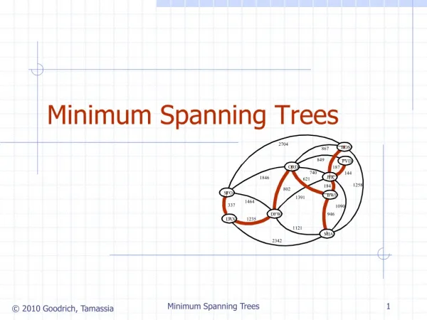
Shortest Path Problem • Given a weighted graph and two vertices u and v, we want to find a path of minimum total weight between u and v. • Length of a path is the sum of the weights of its edges. • Example: • Shortest path between Providence and Honolulu • Applications • Internet packet routing • Flight reservations • Driving directions 849 PVD 1843 ORD 142 SFO 802 LGA 1205 1743 337 1387 HNL 2555 1099 1233 LAX 1120 DFW MIA slide by: Huajie Zhang, http://www.cs.unb.ca/courses/cs3913/

Negative weights • Shortest paths usually undefined for edges with negative weights if there are negative cycles present 2 4 3 -3

Shortest Path Properties Property 1: A subpath of a shortest path is itself a shortest path Property 2: There is a tree of shortest paths from a start vertex to all the other vertices Example: Tree of shortest paths from Providence 849 PVD 1843 ORD 142 SFO 802 LGA 1205 1743 337 1387 HNL 2555 1099 1233 LAX 1120 DFW MIA slide by: Huajie Zhang, http://www.cs.unb.ca/courses/cs3913/

The distance of a vertex v from a vertex s is the length of a shortest path between s and v Dijkstra’s algorithm computes the distances of all the vertices from a given start vertex s Assumptions: the graph is connected the edges are undirected the edge weights are nonnegative We grow a “cloud” of vertices, beginning with s and eventually covering all the vertices We store with each vertex v a label d(v) representing the distance of v from s in the subgraph consisting of the cloud and its adjacent vertices At each step We add to the cloud the vertex u outside the cloud with the smallest distance label, d(u) We update the labels of the vertices adjacent to u Dijkstra’s Algorithm slide by: Huajie Zhang, http://www.cs.unb.ca/courses/cs3913/

Edge Relaxation • Consider an edge e =(u,z) such that • uis the vertex most recently added to the cloud • z is not in the cloud • The relaxation of edge e updates distance d(z) as follows: d(z)min{d(z),d(u) + weight(e)} d(u) = 50 d(z) = 75 10 e u z s d(u) = 50 d(z) = 60 10 e u z s slide by: Huajie Zhang, http://www.cs.unb.ca/courses/cs3913/

0 A 4 8 2 8 2 3 7 1 B C D 3 9 5 8 2 5 E F Example 0 A 4 8 2 8 2 4 7 1 B C D 3 9   2 5 E F 0 0 A A 4 4 8 8 2 2 8 2 3 7 2 3 7 1 7 1 B C D B C D 3 9 3 9 5 11 5 8 2 5 2 5 E F E F slide by: Huajie Zhang, http://www.cs.unb.ca/courses/cs3913/

Example (cont.) 0 A 4 8 2 7 2 3 7 1 B C D 3 9 5 8 2 5 E F 0 A 4 8 2 7 2 3 7 1 B C D 3 9 5 8 2 5 E F slide by: Huajie Zhang, http://www.cs.unb.ca/courses/cs3913/

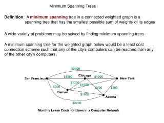
4 10 3 8 2 5 7 9 1 6 Minimum spanning trees • Connect all vertices with a single tree Consider a communications company, such as AT&T or GTE that needs to build a communication network that connects n different users. The cost of making a link joining i and j is cij. What is the minimum cost of connecting all of the users? Common assumption: the only links possible are the ones directly joining two nodes. web.mit.edu/~jorlin/www/15.082/Lectures/16_Spanning_Trees.ppt

2 4 1 3 5 Electronic Circuitry Consider a system with a number of electronic components. In order to make two pins i and j of different components electrically equivalent, one can connect i and j by a wire. How can we connect n different pins in this way to make them electrically equivalent to each other so as to minimize the total wire length. web.mit.edu/~jorlin/www/15.082/Lectures/16_Spanning_Trees.ppt

Minimum Cost Spanning Tree Problem Undirected network G = (N, A). (i, j) is the same arc as (j, i). We associate with each arc (i, j)  A a cost cij. A spanning tree T of G is a connected acyclic subgraph that spans all the nodes. A connected graph with n nodes and n – 1 arcs is a spanning tree. The minimum cost spanning tree problem is to find a spanning tree of minimum cost. web.mit.edu/~jorlin/www/15.082/Lectures/16_Spanning_Trees.ppt

A Minimum Cost Spanning Tree Problem 10 8 2 4 6 35 15 1 17 30 25 20 21 40 3 5 7 15 11 web.mit.edu/~jorlin/www/15.082/Lectures/16_Spanning_Trees.ppt

A Minimum Cost Spanning Tree 10 8 2 4 6 35 15 1 17 30 25 20 21 40 3 5 7 15 11 web.mit.edu/~jorlin/www/15.082/Lectures/16_Spanning_Trees.ppt

Prim-Jarnik Algorithm • Vertex based algorithm • Grows one tree T, one vertex at a time • A cloud covering the portion of T already computed • Label the vertices v outside the cloud with key[v] – the minimum weigth of an edge connecting v to a vertex in the cloud, key[v] = ¥, if no such edge exists www.cs.earlham.edu/~celikeb/fall_2005/cs310_aads/lecture_slides/ch23_minimum_spanning_trees.ppt

Prim Example www.cs.earlham.edu/~celikeb/fall_2005/cs310_aads/lecture_slides/ch23_minimum_spanning_trees.ppt

Prim Example (2) www.cs.earlham.edu/~celikeb/fall_2005/cs310_aads/lecture_slides/ch23_minimum_spanning_trees.ppt

Prim Example (3) www.cs.earlham.edu/~celikeb/fall_2005/cs310_aads/lecture_slides/ch23_minimum_spanning_trees.ppt

Kruskal's Algorithm • The algorithm adds the cheapest edge that connects two trees of the forest MST-Kruskal(G,w) 01A¬Æ 02 for each vertex vÎV[G] do 03 Make-Set(v) 04 sort the edges of E by non-decreasing weight w 05 foreach edge (u,v) ÎE, in order by non-decreasing weight do 06 if Find-Set(u) ¹ Find-Set(v) then 07 A ¬ A È {(u,v)} 08 Union(u,v) 09 return A www.cs.earlham.edu/~celikeb/fall_2005/cs310_aads/lecture_slides/ch23_minimum_spanning_trees.ppt

Kruskal Example www.cs.earlham.edu/~celikeb/fall_2005/cs310_aads/lecture_slides/ch23_minimum_spanning_trees.ppt

Kruskal Example (2) www.cs.earlham.edu/~celikeb/fall_2005/cs310_aads/lecture_slides/ch23_minimum_spanning_trees.ppt

Network flow • Applications • traffic & transportation • maximum number of cars that can commute from Berkley to San Francisco during rush hour • fluid networks: pipes that carry liquids • computer networks: packets traveling along fiber • extended applications (from Kleinberg & Tardos, “Algorithm Design”) • bipartite matching problem • number of disjoint paths between two vertices • survey design • airline scheduling • image segmentation • baseball elimination

Max flow problem: how much stuff can we get from source to sink per unit time? Capacity 7 Sink Source www.comp.nus.edu.sg/~ooiwt/slides/2004-cs3233-graph2.ppt

Equivalent tasks • Find a cut with minimum capacity • Find maximum flow from source to sink www.comp.nus.edu.sg/~ooiwt/slides/2004-cs3233-graph2.ppt

A Flow 3 5 7 2 residual graph 5 2 www.comp.nus.edu.sg/~ooiwt/slides/2004-cs3233-graph2.ppt

SI 614 Directed & weighted networks, minimum spanning trees, flow