
Advanced Statistical Methods for Evaluating Air Quality Models: Beyond Traditional Comparisons
This paper discusses the limitations of standard evaluation methods in air quality modeling, particularly those relying on matched observations and model outputs. We highlight the issues arising from sparse data, measurement errors, and discrepancies between point and volume-averaged observations. Utilizing simulated datasets, we demonstrate how block kriging techniques can address these challenges, providing a more comprehensive spatial evaluation of model outputs. The insights gained from this enhanced analysis can better differentiate between estimation errors and model errors, thus improving air quality assessments.

Advanced Statistical Methods for Evaluating Air Quality Models: Beyond Traditional Comparisons
E N D
Presentation Transcript
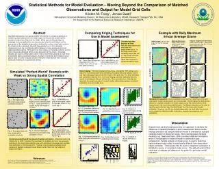
Statistical Methods for Model Evaluation – Moving Beyond the Comparison of Matched Observations and Output for Model Grid Cells Kristen M. Foley1, Jenise Swall1 1Atmospheric Sciences Modeling Division, Air Resources Laboratory, NOAA, Research Triangle Park, NC, USA On Assignment to the National Exposure Research Laboratory, USEPA Abstract Standard evaluations of air quality models rely heavily on a direct comparison of monitoring data matched with the model output for the grid cell containing the monitor's location (e.g. Eder and Yu, 2006). While such techniques may be adequate for many applications, conclusions are limited by such factors as the sparseness of the available observations (limiting the number of grid cells at which the model can be evaluated), potential measurement error in the modeled observations, and the incommensurability between volume-averages and point-referenced observations. While we focus most closely on the latter problem, we find that it cannot be addressed without some discussion of the others. Simulated datasets are used to demonstrate cases in which incommensurability is more likely to adversely affect a traditional analysis. Analysis of observed and modeled ozone data is used to further compare standard evaluation methods and more complex statistical modeling in an operational setting. Comparing Kriging Techniques for Use in Model Assessment Example with Daily Maximum 8-hour Average Ozone Regions of significant differences: Model (CMAQ) output – Observation-based estimates using 95% C.I. from block kriging analysis Matched differences: Model (CMAQ) output – Observations (AIRS, CASTNET sites) Considering other sources of error: Here the observations are simulated with measurement error. In this case, most of the variability around the red 1:1 line comes from the observational errors rather than from the in-commensurability issue. CMAQ output: v4.6 at 12km output for max 8hr average Ozone July 22, 2004 Fig. 7. Observations simulated with measurement error at the locations shown in Fig. 4 (long-range spatial correlation) Fig. 8. Observations vs. grid cell averages, based on the data shown in Fig. 7 and Fig. 5. • Simulated “Perfect-World” Example with Weak vs Strong Spatial Correlation Block kriging: The block kriging technique (e.g., Goovaerts 1997) allows us to adjust for incommensurability by estimating the spatial field at a lattice of points and then averaging these points within each of the grid cells. The error estimates and confidence intervals (C.I.) from block kriging are better calibrated than the results from kriging to the grid cell centers. More accurate error estimates are important for model evaluation in order to better differentiate between statistical estimation error and model error. July 23, 2004 July 24, 2004 Operational evaluation: Using scatterplots such as Fig. 3 and Fig. 6, only grid cells which contain observations can be evaluated. Block kriging the observations allows for a spatial evaluation of model output across the entire domain, while accounting for the incommensurability issue. Confidence intervals can be used to identify regions that are significantly different from the observation-based estimates. However, as with any statistical approach, we must take into account errors related to statistical model formulation, imperfect assumptions and estimation. Fig. 3. Observations vs. grid cell averages, based on the data shown in Fig. 1 and Fig. 2. Fig. 2. Grid cell averages based on the simulated data in Fig. 1. Each grid cell is a square with a side length of 12 units. Fig. 1. Simulated data with short-range spatial correlation structure. Fig. 12. Estimates yielded by kriging the observations in Fig. 7 to the grid cell centers. Fig. 14. Sample of results from kriging to the grid cell centers. Fig. 13. Standard errors yielded by point kriging. Discussion Analysis such as block kriging provides one approach to address the difference in variability between a point measurement and a volume-average prediction by using a statistical model to characterize sub-grid variability based on observed values. More sophisticated statistical modeling, e.g. Swall and Davis, 2006, provides additional information, which is not available in matched model to observation type comparisons. Spatial analysis of model errors is used to determine regions where model output is significantly different from observation-based estimates. These areas may be used for diagnostic evaluation to identify the source of consistent model errors. The added benefit of this extra layer of analysis will depend on the goals of a particular model evaluation. Fig. 6. Observations vs. grid cell averages, based on the data shown in Fig. 4 and Fig. 5. Fig. 5. Grid cell averages based on the simulated data portrayed in Fig.4. Fig. 4. Simulated data with long-range spatial correlation structure. Fig. 15. Estimates yielded by block kriging the observations in Fig 7. Fig. 17. Sample of results from block kriging. Fig. 16. Standard errors yielded by block kriging. Incommensurability and the impact of spatial correlation: Statistical reasoning (Gelfand et al. 2001) indicates that estimates of variability and error are generally sensitive to the incommensurability issue, with estimates of averages less variable than estimates for individual points. However, the discrepancy between point values and spatially averaged values lessens when there is a high degree of spatial correlation. References Eder, B., and S. Yu, 2006: A performance evaluation of the 2004 release of Models-3 CMAQ. Atmos. Envir., 40, 4894-4905. Gelfand, A. E., Zhu, L., and B. P. Carlin, 2001: On the change of support problem for spatio-temporal data, Biostatistics, 2, 31-45. Goovaerts, P. 1997: Geostatistics for Natural Resources Evaluation. Oxford University Press, 483 pp. Swall, J. and J. Davis, 2006: A Bayesian Statistical Approach for Evaluation of CMAQ, Atmos. Envir., 40, 4883-4893. Disclaimer: The research presented here was performed under the Memorandum of Understanding between the U.S. Environmental Protection Agency (EPA) and the U.S. Department of Commerce's National Oceanic and Atmospheric Administration (NOAA) and under agreement number DW13921548. This work constitutes a contribution to the NOAA Air Quality Program. Although it has been reviewed by EPA and NOAA and approved for publication, it does not necessarily reflect their policies or views.


