Download
1 / 44
440 likes | 545 Vues
This study presents a detailed analysis of the KL lifetime measurement, focusing on the neutral vertex algorithm and χ2 minimization method. The data sample and MC sample are thoroughly evaluated to minimize the residuals and determine the KL decay path efficiently.

E N D
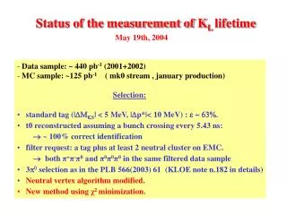
Status of the measurement of KL lifetime May 19th, 2004 • Data sample: ~ 440 pb-1 (2001+2002) • MC sample: ~125 pb-1 ( mk0 stream , january production) • Selection: • standard tag (|DMKS| < 5 MeV, |Dp*|< 10 MeV) : e ~ 63%. • t0 reconstructed assuming a bunch crossing every 5.43 ns: • ~ 100% correct identification • filter request: a tag plus at least 2 neutral cluster on EMC. • both π+π-π0 and π0π0π0 in the same filtered data sample • 3p0 selection as in the PLB 566(2003) 61 (KLOE note n.182 in details) • Neutral vertex algorithm modified. • New method using χ2 minimization.
Lkn Lki Lki-1 <Lk> “Modified” neutral vertex algorithm: 1) Select events with a vertex in DC and 2 clusters not associated to tracks. 2) For each neutral cluster build a Lki. 3) Order the Lki in ascending order along the KL flight direction 4) Look for the closest 2 Lk that satisfy |Lk2- Lk1| < 6 σ1γ and build the weighted average. 5) Go ahead and behind to look for other clusters that satisfy: |Lki – <LK >| < 6 σtot , σtot = σ1γ σ2γ 6) The event is kept if there is at least a third cluster in time with the closest two (MC probability ~ 99.4%) (validation). Now I can use the KLπ+π-π0 sample to evaluate everything
residuals: KL decay path: (fit-data)/fit ±0.5% 0.38% stat Fit region: 50–158 cm
KL decay path (II): Lk fit vs Lmin χ2 vs Lmin Lmin
Lk fit vs Lmax KL decay path (III): χ2 vs Lmax Lmax
New method:χ2 minimization • Define χ2 as: • For each event build χ2 and minimize it by moving LK 0 from –5 cm to +5 cm around the starting value. • The starting value has been chosen as the weighted average of the two closest clusters.
LK0 ranges from –5 cm to + 5 cm around the starting value: χ2 distribution: data MC data MC The χ2 is minimum at the starting value χ2 method (II):
LK (fit) χ2 method (III): Lmin LK (fit) Lmax
Comparison between different methods in the same fit region (50-158 cm): Weighted average with the 2 closest photons 341.2 ± 1.3 cm 54/53 Weighted average using all the photons: 340.9 ± 1.3 cm 53/53 χ2 method : 340.8 ± 1.3 cm 50/53 Most energetic cluster : 343.4 ± 1.4 cm 115/53
Background analysis (I): remaining background ~ 1.2% (mainly from 4 γ sample)
N=4 Background distributes uniformely along decay region Background analysis (II):
LK = βγcτ β (KL) (lab) β (KL) (cdm)
Result: τ (KL) = (51.15 ±0.2) ns residuals 7.5 ns (50 cm) 23.6 ns (158 cm) t (PDG) (fit) = (51.7 ± 0.4) ns t (Vosburg, 1972) = (51.54 ± 0.44) ns - 0.4 Mevents (PRD 6 (1972), 1834) t (KLOE) = (51.15 ± 0.2 stat ) ns - 14.5 Mevents – 440 pb-1
Lifetime with a fixed number of clusters: We have to use all the photons if we want to avoid acceptance corrections
Lifetime with a fixed number of clusters (data-MC comparison): N=3 ( 0.6%) N=4 ( 9.2%) Fit region Fit region N=5 (31.4%) N=6 (55.8%) Fit region Fit region
Lifetime with a fixed number of clusters (data-MC comparison): N=8 (~0.1%) N=7 (~3%) • For N=7 and N=8 populations there is a bump at Lk ~ 30 cm not observed in MC. • MC was not corrected for discriminator threshold and merging.
Lifetime with a fixed number of clusters (data-MC comparison): z (cm) Rt (cm)
Sample with 7 photons: All the photons are in-time The total energy is OK Etot (MeV) Tγ – TK (ns)
Cluster multeplicity in different zones of FV: 40 cm < Rt < 160 cm (ALL) 40 cm < Rt < 80 cm (first zone) 120 cm < Rt < 160 cm (third zone) 80 cm < Rt < 120 cm (second zone) Discrepancy due to different cluster thresholds in DATA-MC
To do: • Filter new Monte Carlo production and put threshold on MC clusters: 1) to check cluster multeplicities distributions; 2) to understand the nature of the bump in decay distributions for N=7 and N=8 populations; 3) to check behaviour of decay distributions near inner wall (regeneration zone). • Remove π0π0 and γγ background through cut on invariant mass. • Evaluate how much are close the two closest clusters for 3π0 and π+π-π0 samples as a function of Lk. •Evaluate vertex reconstruction efficiency using the χ2 method with the π+π-π0 sample. • …………………………
Conclusions: • Full data sample analysed (~ 440 pb-1). • Decay vertex reconstructed using the weighted average of the two closest • photons. • New method (χ2 minimization) confirms validity of weighted averages • algorithms. • Vertex reconstruction efficiency variations evaluated using π+π-π0 • data sample. • Fit region defined as the maximum range with minimum efficiency • variations and minimum spread of the residuals: • • Statistical error in fit region is 0.38%.
Experiment performed at Princeton Pennsylvania Accelerator where KL beam was created at 90° with respect to the 3 GeV proton beam incident on Pt target. The beam has a pronounced time structure : each bunch is ~1 ns wide and separated from the others by ~ 33 ns: this time structure is used to determine TOF of decaying particles ( KOPIO’s method ). Detector and collimator were mounted on carts that were moved of ~ 24 m corresponding to 1.5-3.7 mean lives of KL in the momentum range detected (150-500 MeV) The data taking consists of 6 different runs at 6 different positions (different acceptance, different momentum range of Kaons,..) for a total of 0.4 Mevents collected. The detector consists in 4 telescopes placed around the vacuum chamber and consist of two 1.28 cm plastic scintillators separated by 0.6 cm steel plate + cosmic vetos. A telescope is considered if there is a coincidence between signals of the two inner scintillator counters: if two or more telescope are fired in absence of any cosmic-ray veto counter the signal is kept and used for TOF measurement. Only flux of protons can be measured: monitors were sensitive in A different way to the number of protons striking the production target. The normalization procedure rests on the assumption that the KL flus is proportional to the rate of these monitors for a given momentum of the primary proton beam. Old measurement of KL lifetime:
The number of KL decays is: N (D,P) = N0 (P) ε (D,P) Ω(D) exp(-MD/Pτ) Where N0(P) = is the production intensity (from protons monitors) Ω(D) = solid angle subtended by the detector (evaluated using Monte Carlo) ε (D,P) = efficiency (evaluated using Monte Carlo) Lifetime is obtained through a least squares fit which determines also a set of 9 parameters that describe the kaon production spectrum at the synchrotron target After multiplication bu the efficiency for detecting a kaon in the apparatus. The explicit form of the χ2 is: Where j runs on the 6 runs, k runs on the momentum bins, Wjk =1, 0 if the bin is considered or not, Kij is the normalized detected kaon rate Δjk is its uncertainty, Fjk is the N(D,P) for each momentum bin (here enters the 9 parameters needed to fit the momentum spectrum).
Considerations and open questions: • - The main characteristic of this decay is to have a large number of photons • and the strong point of this analysis is to keep (almost) all the photons that are • produced (N 3) . • This method makes the effects of the cluster reconstruction efficiency • and the acceptance very small. • Two things must be taken under control: • 1) the background; • 2) the variation of the reconstruction efficiency of the decay vertex • with the decay path. is it possibile to use data in some way?
1) Vertex reconstruction efficiency MC:ε (<Lγγ>) vs LK (true) DATA:ε (<Lγγ>) vs LK (π+π-) DATA: π+π-π0 “selected” MC: π+π-π0 “true” MC: π+π-π0 “selected” LK (true) (cm) LK (π+π-) (cm)
KL π+π-π0 selection (I): The selection criteria must not bias the vertex reconstruction efficiency Cut on the charged sector: Cut on the neutral sector: Pmiss- Emiss E(π0)(expected) – E(π0)(γγ)
KL π+π-π0 selection (II): Background: Control plot: Background ~ 1 % M (π0) from the best two γ
2) Resolutions: KL +-0 data sample σ(1γ) σ(2γ)
3) Weighted Average: With the KL π+π-π0 sample we can check the 1/(E) behavior: σ(LK) vs LK (π+π-) σ(LK) vs Eγ
“Standard” neutral vertex algorithm: 1) for each neutral cluster build a Lk 2) order the Lk in ascending order along the KL flight direction 3) look for the closest 3 Lk that satisfy |Lk3- Lk1| < 6 σ1γ 4) If found, build <Lk>. 5) Look ahead and behind if there are other Lki that satisfy |Lki - <LK>| < 6 σ tot σ tot = σ (<L>) σ (1γ) 6) Build the weighted average with all the photons that satisfy these criteria. No way to test reconstruction efficiency uniformity using data (no control sample with 3 photons). Lkn Lki Lki-1 <Lk>
First attempt: try to use the most energetic photon in the event Advantage: I can use the KL π+π-π0 sample to check the variation of the vertex reconstruction efficiency with the decay path. Disadvantage: I loose resolution (but for lifetime is not so critical….)
1) Decay path recontructed using the most energetic photon fit region: 35 cm – 165 cm (fit-data)/fit ±1% more data than foreseen… ..regeneration? background? efficiency? - If I use the most energetic photon I cannot avoid background. - Background is mainly concentrated at low LK. - The rejection of background introduces again some dependency of the efficiency with Lk (which makes the idea useless).
KL decay path (IV): Check if the π0π0π0 selection introduces some bias in the lifetime MC before selection: MC after selection: The two results are in agreement within the errors Lk(true) Lk(true)
Cluster multeplicity: Cluster energy: DATA QUALITY (I):
Total energy for N = 3 Total energy for N = 4 DATA QUALITY (II)
Total energy for N = 6 Total energy for N = 5 Total energy for N=8,9,… Total energy for N=7 DATA QUALITY (III)
Lk dal cluster piu’ energetico tra quelli selezionati da twogam: (id=412)
Lk dalla media pesata tra quelli selezionati da twogam: (id=416)